Case Study 2 DDS
Matt Sherga
8/15/2020
Description:
DDSAnalytics has requested an analysis of employee data with the intent to decrease the rate of attrition, as well as form a model for predicting attrition, and another model for predicting monthly income based on whatever factors are found to be influential. Additional analysis is welcome.
Analyze existing employee data at DDSAnalytics to:
- Predict employee Attrition
- Identify any Job-Role specific trends
- Determine the top three most influential factors that contribute to Attrition
- Establish criteria for predicting monthly income, and create a regression model
Process:
First, the data was cleaned and organized. There were no missing values, and the data was comprised of both categorical and continuous variables. The categories “EmployeeCount”, “Over18”, and “StandardHours” all only had one level so they were removed from the data.
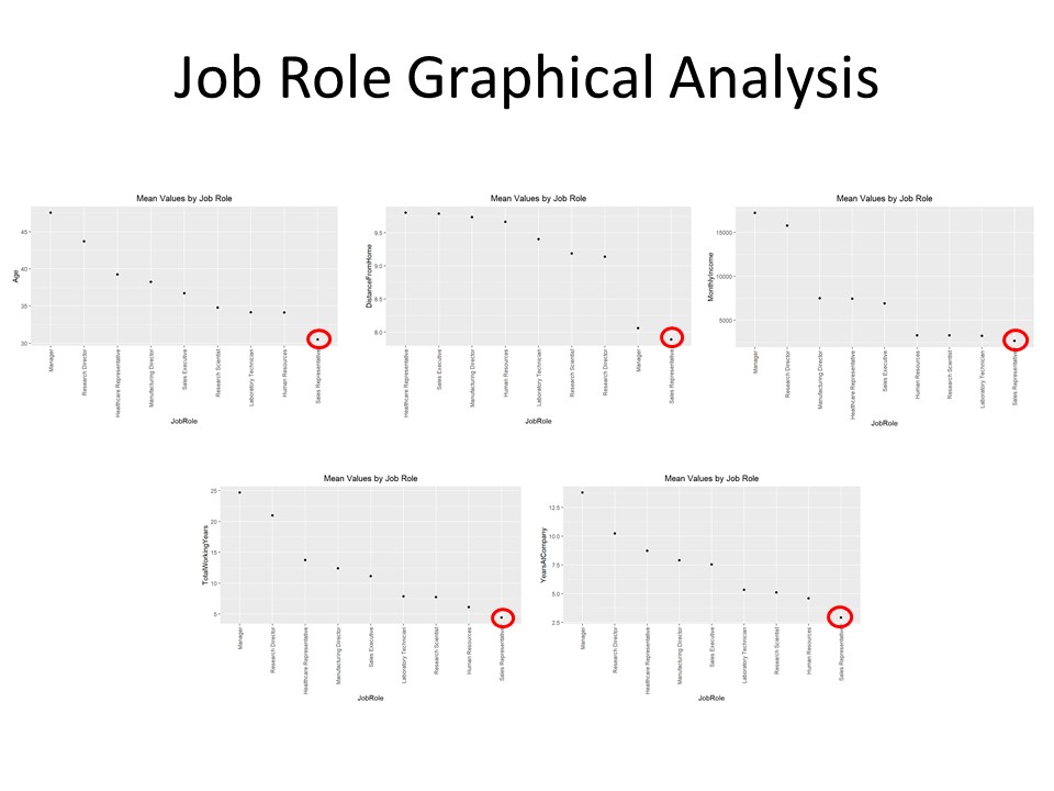
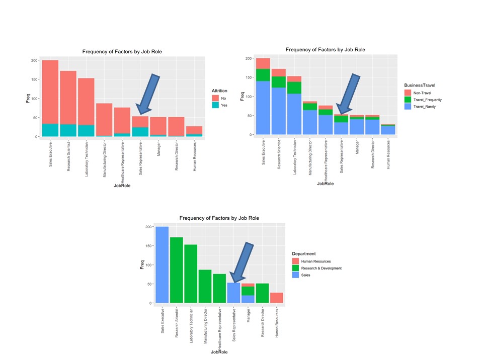
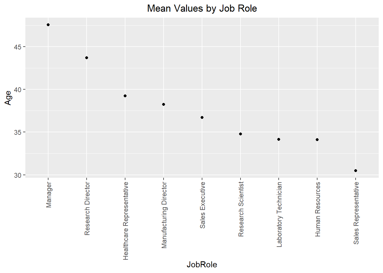
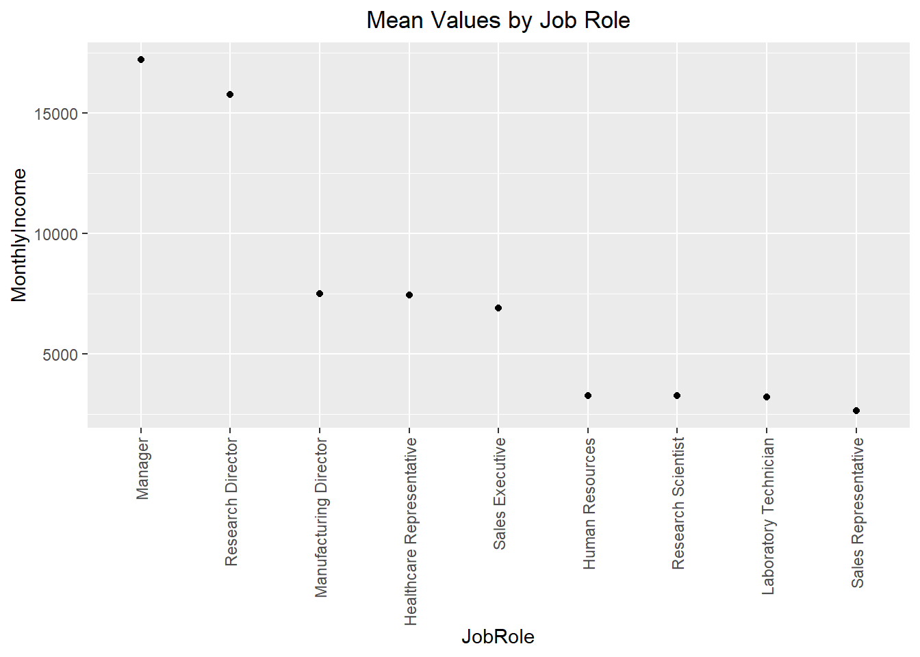
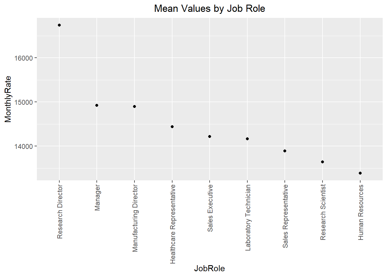
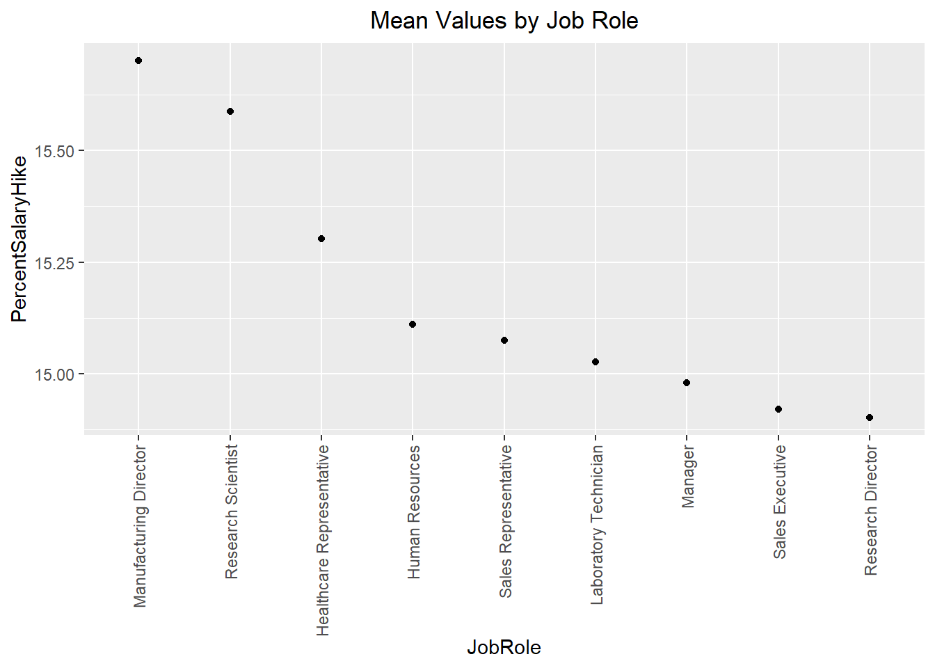
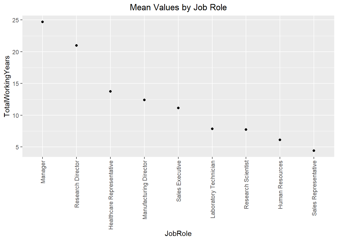
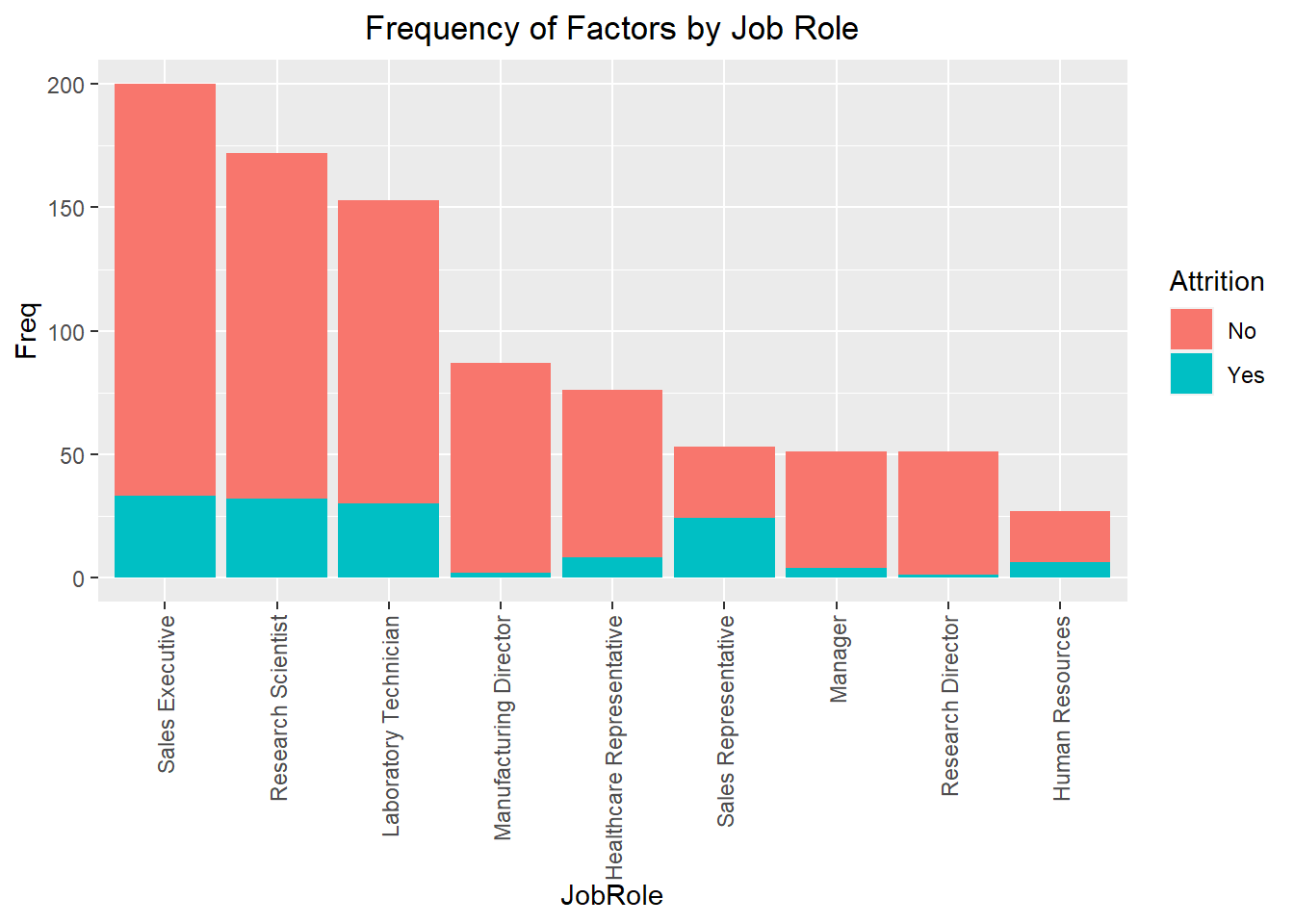
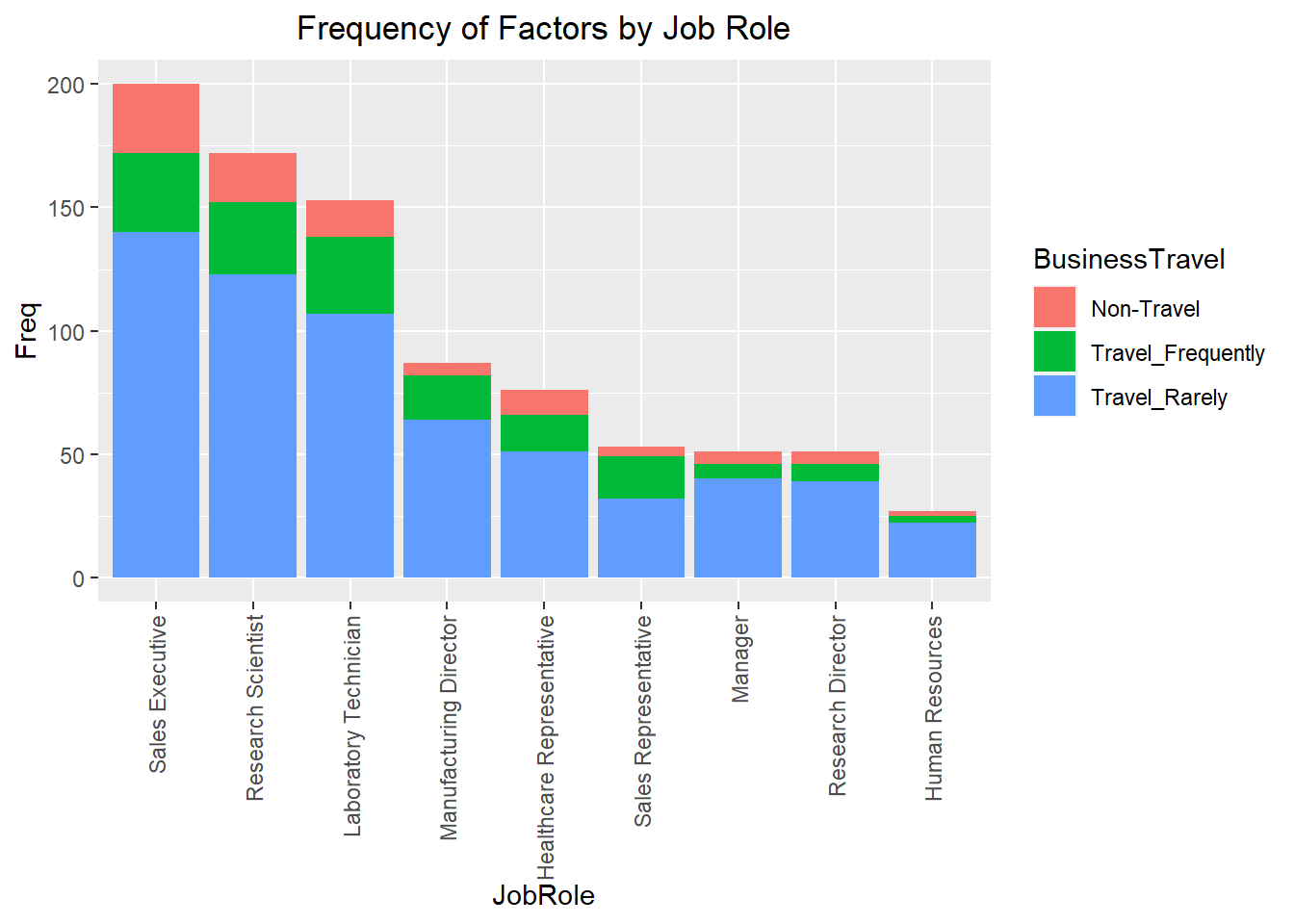
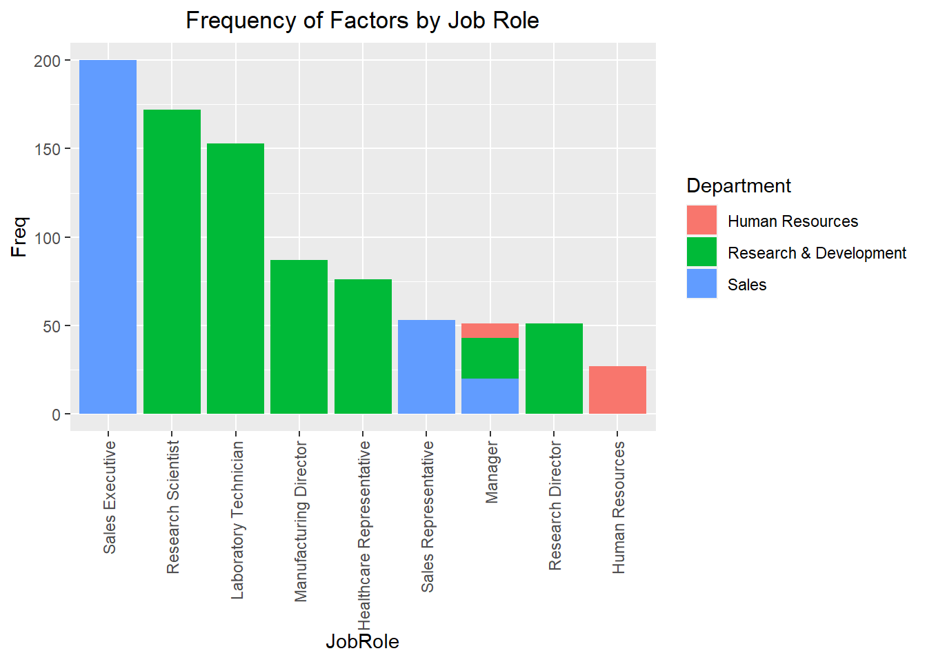
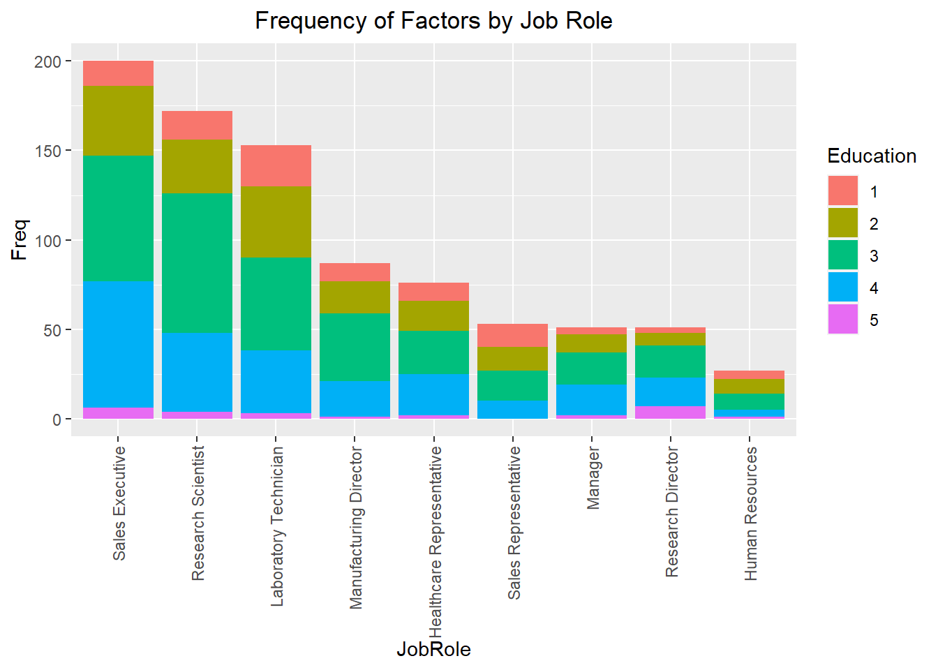
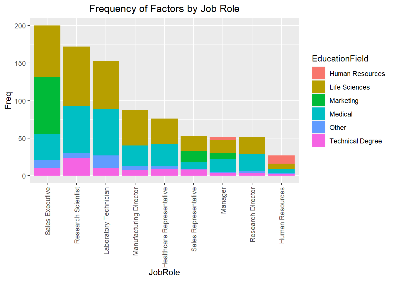
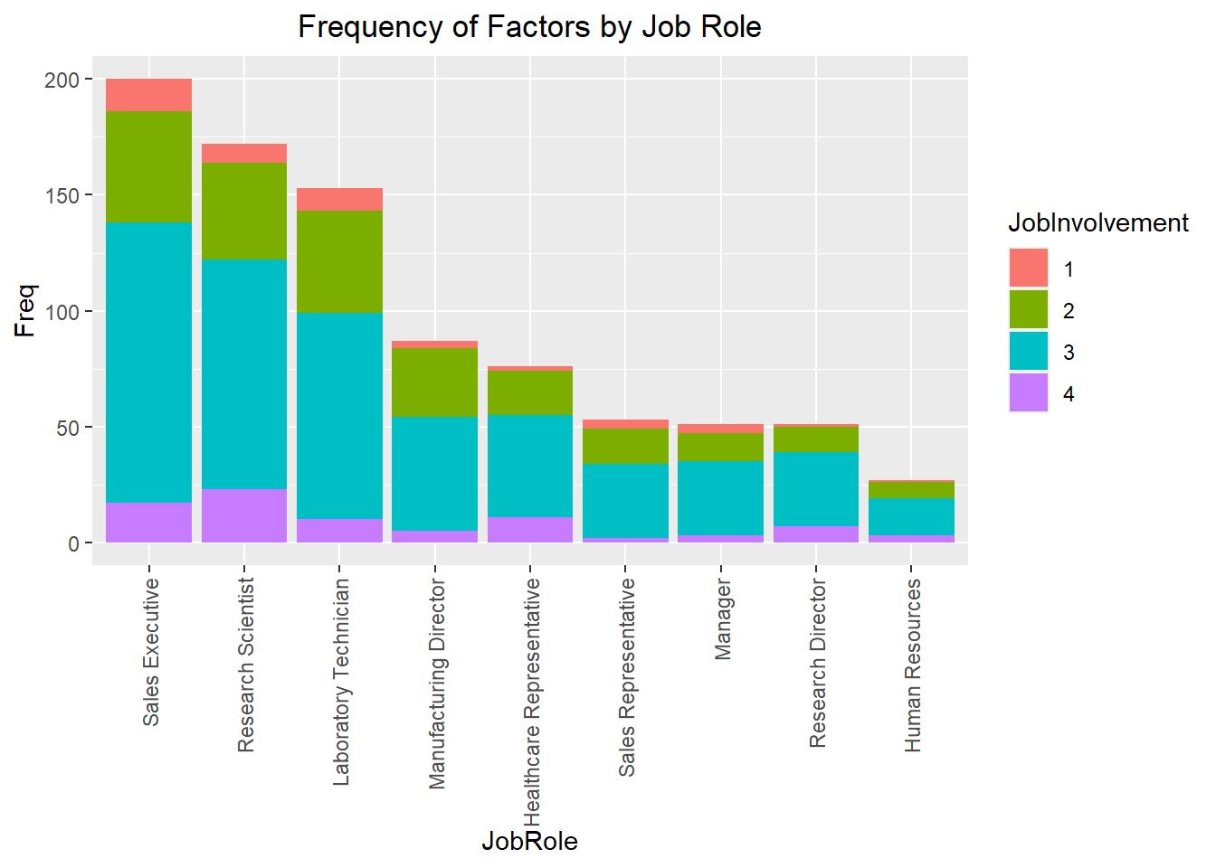
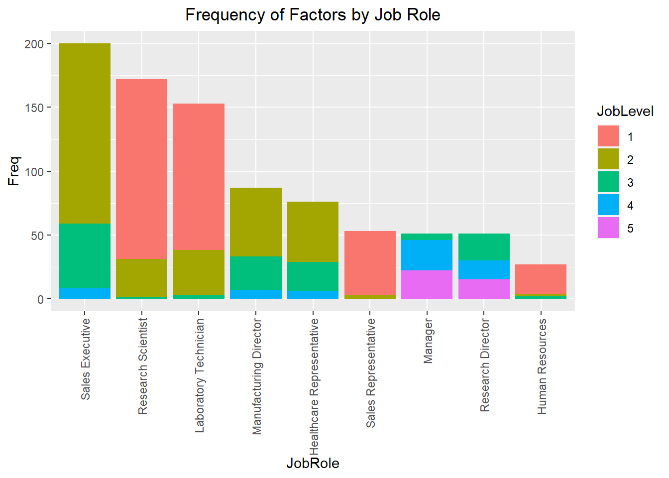
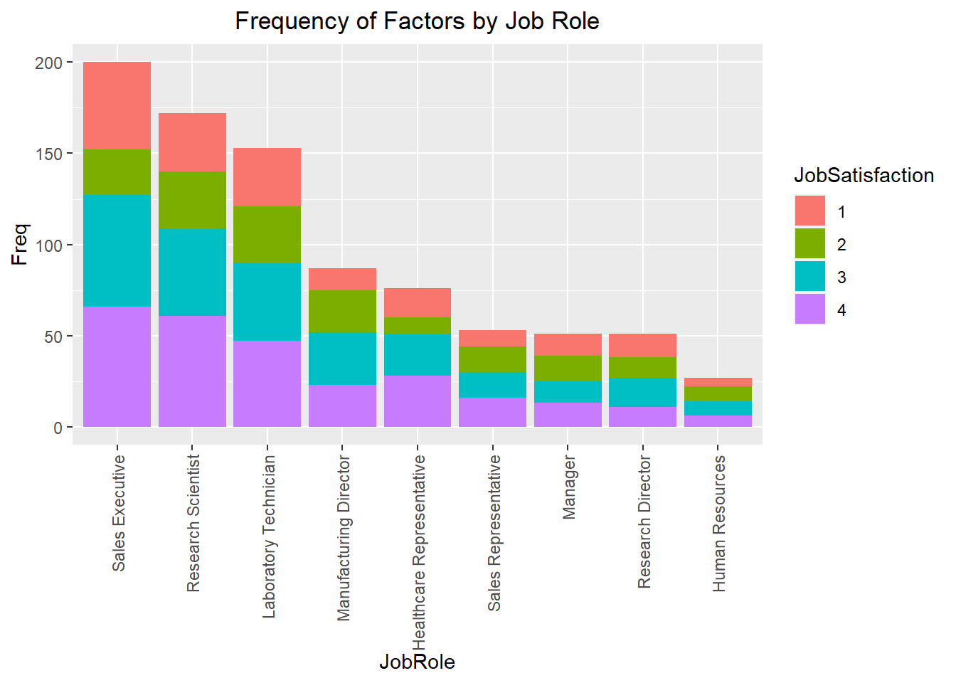
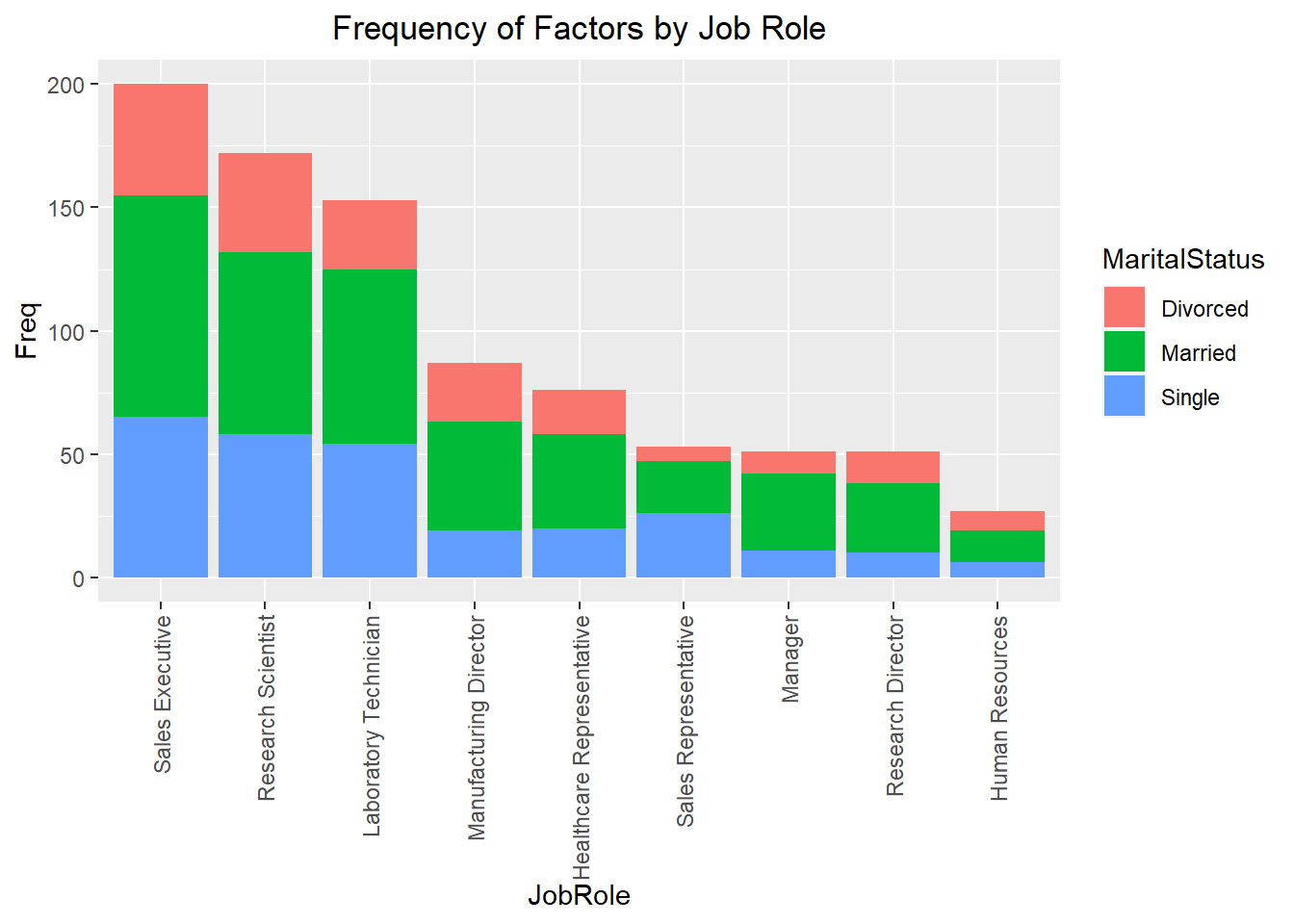
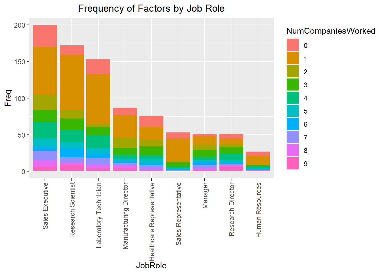
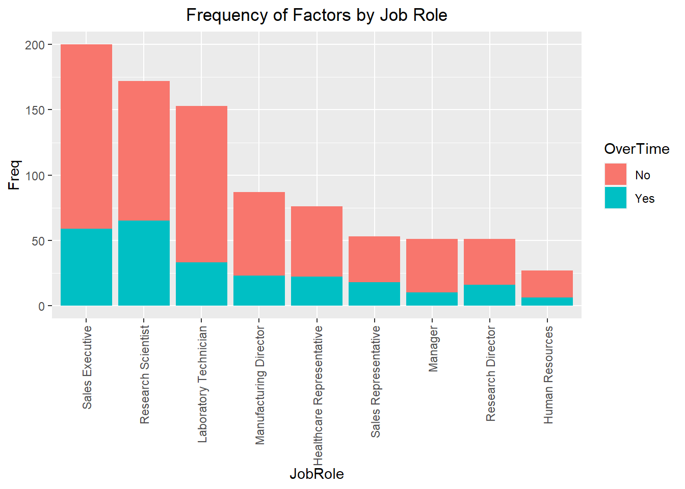
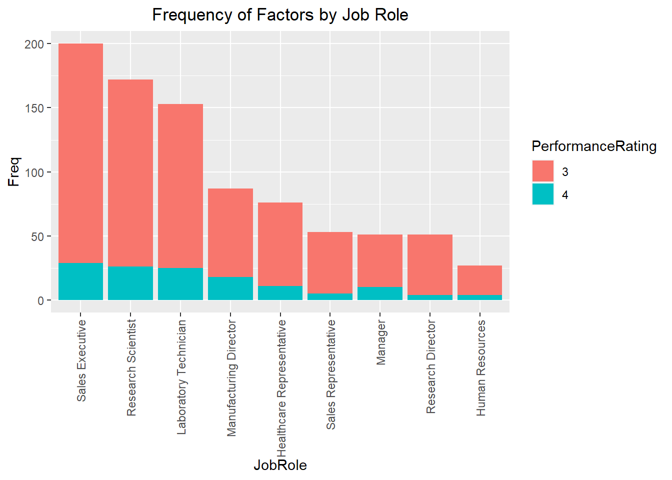
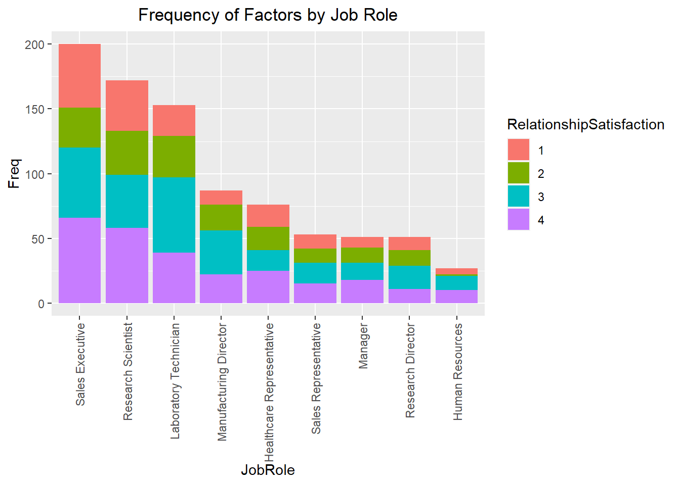
Next, the mean of each continuous variable, and a frequency bar chart for categories, were plotted according to Job Role. Sales Representatives are, on average, the youngest, live closest to work, the lowest monthly income, fewest working years, and fewest years at the company. When looking at attrition, you can see that they also have the highest rate of departures compared to any other job role (almost 50%). If you take a look at business travel, a substantial percentage of sales reps travel frequently when compared to other roles. Sales representatives make up a relatively small portion of the Sales department, especially when compared to Sales Executives. This may be due to the higher rate of attrition in that role, but at a lower income it seems like you might get value at accelerating hiring of this role.
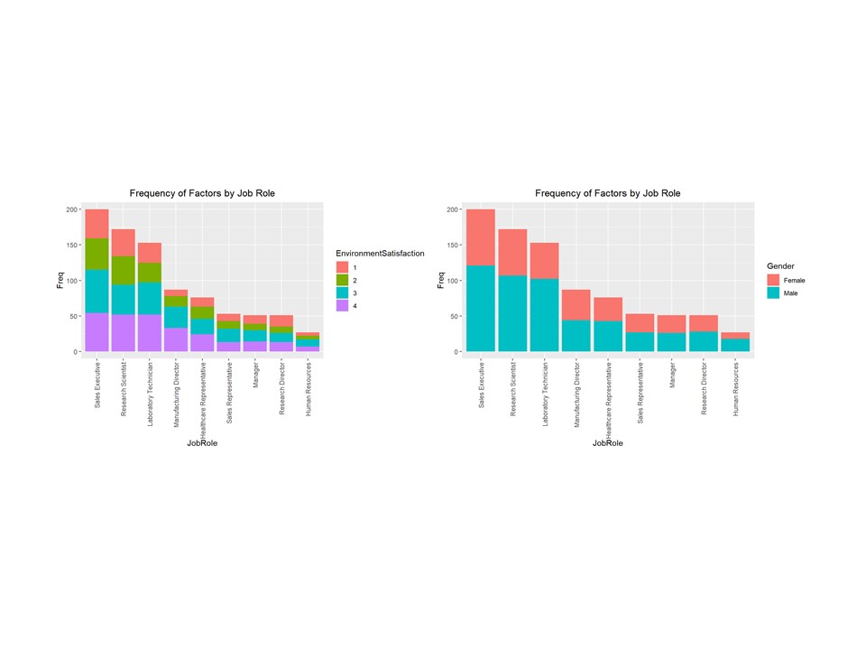
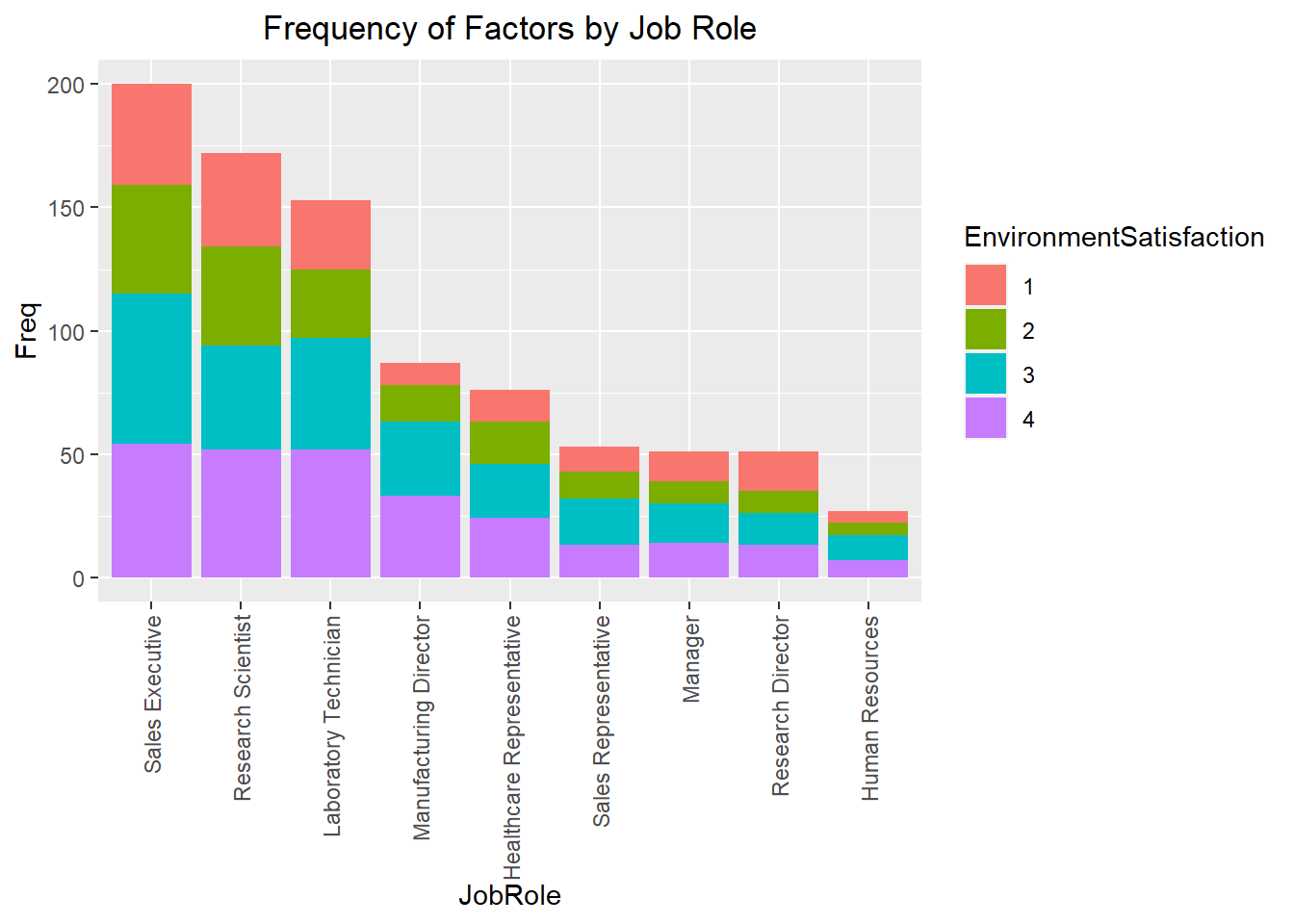
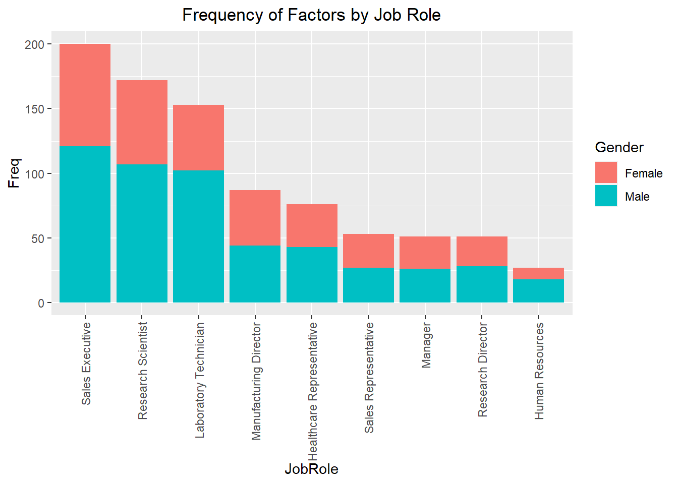
Environment Satisfaction scores were mostly evenly distributed within and across every job role. You also look to have good gender diversity across all job roles, although research scientists and lab techs look to be slightly higher percentage male, as does human resources.
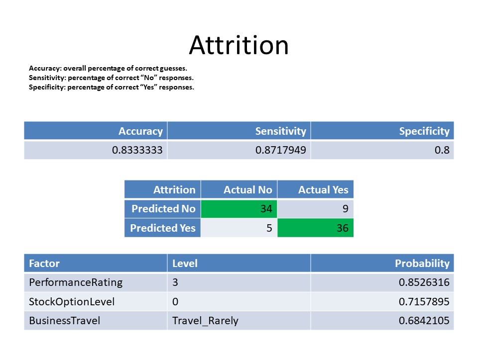
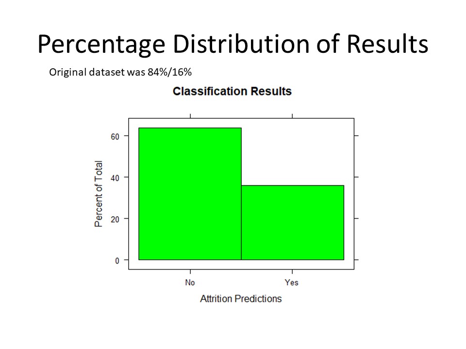
The data was heavily skewed toward “No” for attrition, so it was randomly subsampled to compare with less bias. A best seed was found for creating test and train samples, and Naïve Bayes was run on the data. It was found that the top three highest probability Attrition factors are employees who Travel Rarely (conditional prob = .68), Stock Option level of 0 (cp = .71), and performance rating of 3 (cp = .85). The model we created had an accuracy of .833, Sensitivity of .871, and Specificity of .800 when run against the test set. When used to predict attrition for the competition data, the outcome was again heavily skewed toward “no” attrition. So if that data sample is representative of our starting dataset, this reinforces our model.
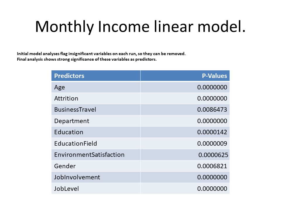
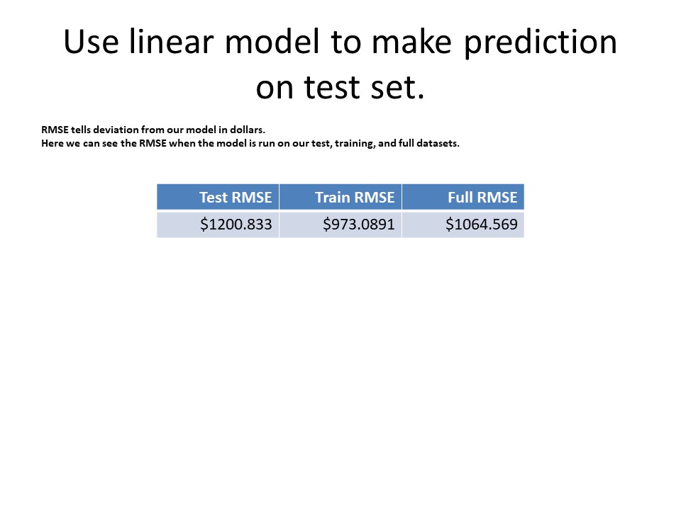
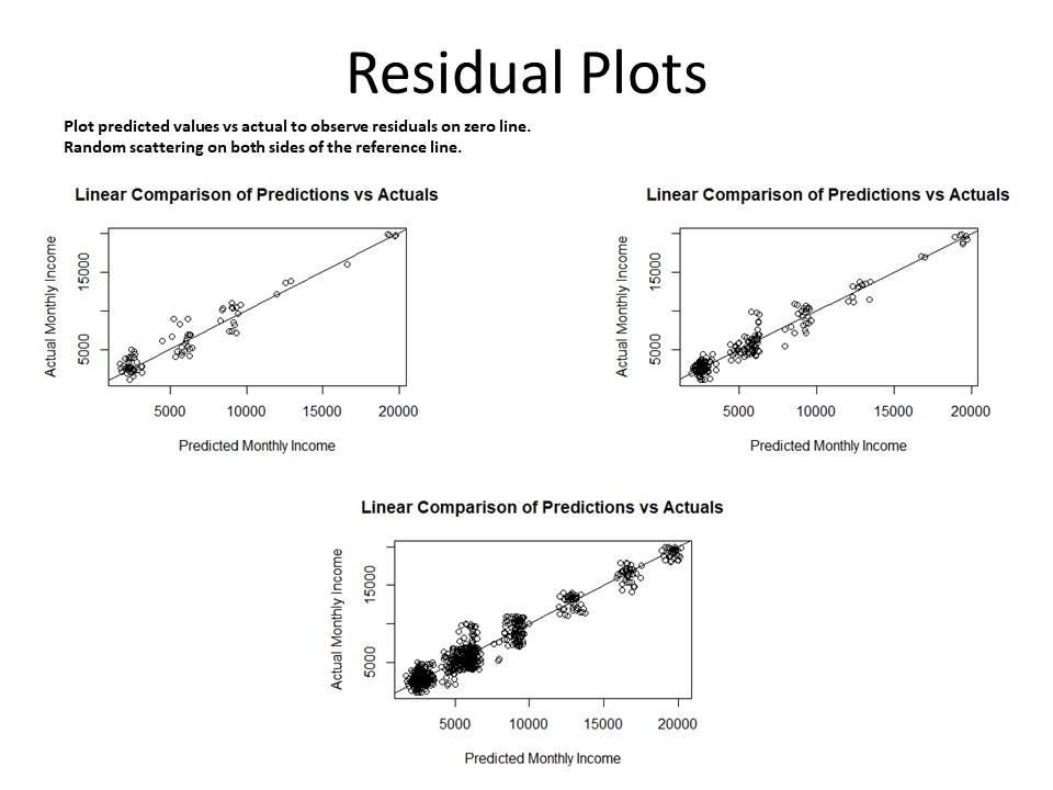
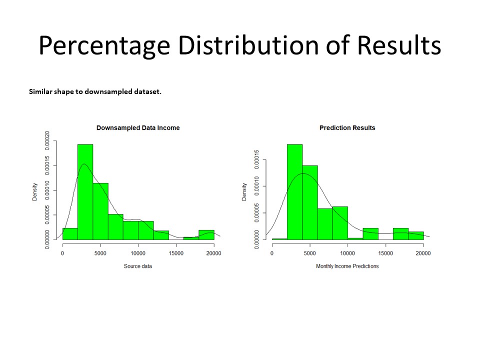
For our second model, we set out to determine what factors can be used to predict monthly income. Again, the data was split into a training and test set, and this time we ran linear regression against all variables. An ANOVA was run to determine what variables are significant predictors in our model. We then re-ran the regression, and ANOVA until all our predictors had significant p-values < .05. Age, Attrition, Business Travel, Department, Education, EducationField, EnvironmentSatisfaction, Gender, JobInvolvement, JobLevel, and JobRole were all deemed significant in our model. Each had a p-value <.001 except for business travel with a .008. The model was run against the test set, the train set, and the full dataset to receive respective RMSE values of $1200.83, $973.09, and $1064.57. We then created residual plots for each of these, and see that the data is randomly scattered along the zero line with no influential points. Finally, density plots were compared between the predictions on the competition sets, and on the downsampled data. They have very similar shapes, which reinforces the strength of the model.
# Load the libraries in R
library(MASS)
library(ggplot2)
library(dplyr)
library(e1071)
library(caret)
library(psych)
library(Amelia)#missmap for graphing missing values
library(broom) #tidy
library(DescTools)
library(car) #outliertest
library(readxl)
library(knitr)#nicer tables for ppt
library(rminer)#variable importance for NB
library(rms)
library(GGally)
library(tidyverse)
EDA How does the dataset look?
No missing values
EmployeeNumber was not removed because I do not know if there is a system to assigning them. It may have some meaning I’m unaware of.
# Set global seed. Load the dataset from the file system and convert appropriate columns to factors, and remove factors with only one level.
set.seed(123)

df1 <- read.csv("CaseStudy2-data.csv")
#any missing data? no
missmap(df1)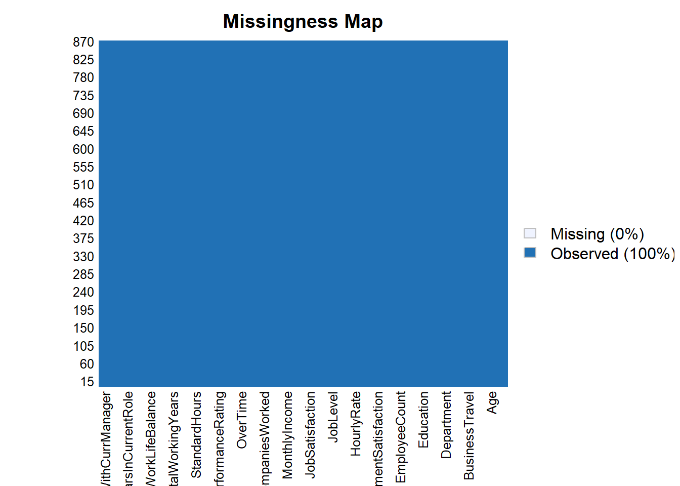
What data is categorical?
#learn more about it
str(df1)
## 'data.frame': 870 obs. of 36 variables:
## $ ID : int 1 2 3 4 5 6 7 8 9 10 ...
## $ Age : int 32 40 35 32 24 27 41 37 34 34 ...
## $ Attrition : chr "No" "No" "No" "No" ...
## $ BusinessTravel : chr "Travel_Rarely" "Travel_Rarely" "Travel_Frequently" "Travel_Rarely" ...
## $ DailyRate : int 117 1308 200 801 567 294 1283 309 1333 653 ...
## $ Department : chr "Sales" "Research & Development" "Research & Development" "Sales" ...
## $ DistanceFromHome : int 13 14 18 1 2 10 5 10 10 10 ...
## $ Education : int 4 3 2 4 1 2 5 4 4 4 ...
## $ EducationField : chr "Life Sciences" "Medical" "Life Sciences" "Marketing" ...
## $ EmployeeCount : int 1 1 1 1 1 1 1 1 1 1 ...
## $ EmployeeNumber : int 859 1128 1412 2016 1646 733 1448 1105 1055 1597 ...
## $ EnvironmentSatisfaction : int 2 3 3 3 1 4 2 4 3 4 ...
## $ Gender : chr "Male" "Male" "Male" "Female" ...
## $ HourlyRate : int 73 44 60 48 32 32 90 88 87 92 ...
## $ JobInvolvement : int 3 2 3 3 3 3 4 2 3 2 ...
## $ JobLevel : int 2 5 3 3 1 3 1 2 1 2 ...
## $ JobRole : chr "Sales Executive" "Research Director" "Manufacturing Director" "Sales Executive" ...
## $ JobSatisfaction : int 4 3 4 4 4 1 3 4 3 3 ...
## $ MaritalStatus : chr "Divorced" "Single" "Single" "Married" ...
## $ MonthlyIncome : int 4403 19626 9362 10422 3760 8793 2127 6694 2220 5063 ...
## $ MonthlyRate : int 9250 17544 19944 24032 17218 4809 5561 24223 18410 15332 ...
## $ NumCompaniesWorked : int 2 1 2 1 1 1 2 2 1 1 ...
## $ Over18 : chr "Y" "Y" "Y" "Y" ...
## $ OverTime : chr "No" "No" "No" "No" ...
## $ PercentSalaryHike : int 11 14 11 19 13 21 12 14 19 14 ...
## $ PerformanceRating : int 3 3 3 3 3 4 3 3 3 3 ...
## $ RelationshipSatisfaction: int 3 1 3 3 3 3 1 3 4 2 ...
## $ StandardHours : int 80 80 80 80 80 80 80 80 80 80 ...
## $ StockOptionLevel : int 1 0 0 2 0 2 0 3 1 1 ...
## $ TotalWorkingYears : int 8 21 10 14 6 9 7 8 1 8 ...
## $ TrainingTimesLastYear : int 3 2 2 3 2 4 5 5 2 3 ...
## $ WorkLifeBalance : int 2 4 3 3 3 2 2 3 3 2 ...
## $ YearsAtCompany : int 5 20 2 14 6 9 4 1 1 8 ...
## $ YearsInCurrentRole : int 2 7 2 10 3 7 2 0 1 2 ...
## $ YearsSinceLastPromotion : int 0 4 2 5 1 1 0 0 0 7 ...
## $ YearsWithCurrManager : int 3 9 2 7 3 7 3 0 0 7 ...describe(df1)## df1
##
## 36 Variables 870 Observations
## --------------------------------------------------------------------------------
## ID
## n missing distinct Info Mean Gmd .05 .10
## 870 0 870 1 435.5 290.3 44.45 87.90
## .25 .50 .75 .90 .95
## 218.25 435.50 652.75 783.10 826.55
##
## lowest : 1 2 3 4 5, highest: 866 867 868 869 870
## --------------------------------------------------------------------------------
## Age
## n missing distinct Info Mean Gmd .05 .10
## 870 0 43 0.999 36.83 10.07 24 26
## .25 .50 .75 .90 .95
## 30 35 43 50 54
##
## lowest : 18 19 20 21 22, highest: 56 57 58 59 60
## --------------------------------------------------------------------------------
## Attrition
## n missing distinct
## 870 0 2
##
## Value No Yes
## Frequency 730 140
## Proportion 0.839 0.161
## --------------------------------------------------------------------------------
## BusinessTravel
## n missing distinct
## 870 0 3
##
## Value Non-Travel Travel_Frequently Travel_Rarely
## Frequency 94 158 618
## Proportion 0.108 0.182 0.710
## --------------------------------------------------------------------------------
## DailyRate
## n missing distinct Info Mean Gmd .05 .10
## 870 0 627 1 815.2 463.3 175.4 257.8
## .25 .50 .75 .90 .95
## 472.5 817.5 1165.8 1368.0 1436.7
##
## lowest : 103 111 117 119 120, highest: 1490 1495 1496 1498 1499
## --------------------------------------------------------------------------------
## Department
## n missing distinct
## 870 0 3
##
## Value Human Resources Research & Development Sales
## Frequency 35 562 273
## Proportion 0.040 0.646 0.314
## --------------------------------------------------------------------------------
## DistanceFromHome
## n missing distinct Info Mean Gmd .05 .10
## 870 0 29 0.993 9.339 8.843 1.0 1.0
## .25 .50 .75 .90 .95
## 2.0 7.0 14.0 23.1 26.0
##
## lowest : 1 2 3 4 5, highest: 25 26 27 28 29
## --------------------------------------------------------------------------------
## Education
## n missing distinct Info Mean Gmd
## 870 0 5 0.917 2.901 1.12
##
## lowest : 1 2 3 4 5, highest: 1 2 3 4 5
##
## Value 1 2 3 4 5
## Frequency 98 182 324 240 26
## Proportion 0.113 0.209 0.372 0.276 0.030
## --------------------------------------------------------------------------------
## EducationField
## n missing distinct
## 870 0 6
##
## lowest : Human Resources Life Sciences Marketing Medical Other
## highest: Life Sciences Marketing Medical Other Technical Degree
##
## Value Human Resources Life Sciences Marketing Medical
## Frequency 15 358 100 270
## Proportion 0.017 0.411 0.115 0.310
##
## Value Other Technical Degree
## Frequency 52 75
## Proportion 0.060 0.086
## --------------------------------------------------------------------------------
## EmployeeCount
## n missing distinct Info Mean Gmd
## 870 0 1 0 1 0
##
## Value 1
## Frequency 870
## Proportion 1
## --------------------------------------------------------------------------------
## EmployeeNumber
## n missing distinct Info Mean Gmd .05 .10
## 870 0 870 1 1030 698.6 86.9 191.1
## .25 .50 .75 .90 .95
## 477.2 1039.0 1561.5 1856.2 1958.3
##
## lowest : 1 4 11 13 14, highest: 2041 2053 2056 2062 2064
## --------------------------------------------------------------------------------
## EnvironmentSatisfaction
## n missing distinct Info Mean Gmd
## 870 0 4 0.93 2.701 1.22
##
## Value 1 2 3 4
## Frequency 172 178 258 262
## Proportion 0.198 0.205 0.297 0.301
## --------------------------------------------------------------------------------
## Gender
## n missing distinct
## 870 0 2
##
## Value Female Male
## Frequency 354 516
## Proportion 0.407 0.593
## --------------------------------------------------------------------------------
## HourlyRate
## n missing distinct Info Mean Gmd .05 .10
## 870 0 71 1 65.61 23.24 34 39
## .25 .50 .75 .90 .95
## 48 66 83 94 97
##
## lowest : 30 31 32 33 34, highest: 96 97 98 99 100
## --------------------------------------------------------------------------------
## JobInvolvement
## n missing distinct Info Mean Gmd
## 870 0 4 0.775 2.723 0.7042
##
## Value 1 2 3 4
## Frequency 47 228 514 81
## Proportion 0.054 0.262 0.591 0.093
## --------------------------------------------------------------------------------
## JobLevel
## n missing distinct Info Mean Gmd
## 870 0 5 0.896 2.039 1.139
##
## lowest : 1 2 3 4 5, highest: 1 2 3 4 5
##
## Value 1 2 3 4 5
## Frequency 329 312 132 60 37
## Proportion 0.378 0.359 0.152 0.069 0.043
## --------------------------------------------------------------------------------
## JobRole
## n missing distinct
## 870 0 9
##
## lowest : Healthcare Representative Human Resources Laboratory Technician Manager Manufacturing Director
## highest: Manufacturing Director Research Director Research Scientist Sales Executive Sales Representative
##
## Healthcare Representative (76, 0.087), Human Resources (27, 0.031), Laboratory
## Technician (153, 0.176), Manager (51, 0.059), Manufacturing Director (87,
## 0.100), Research Director (51, 0.059), Research Scientist (172, 0.198), Sales
## Executive (200, 0.230), Sales Representative (53, 0.061)
## --------------------------------------------------------------------------------
## JobSatisfaction
## n missing distinct Info Mean Gmd
## 870 0 4 0.929 2.709 1.236
##
## Value 1 2 3 4
## Frequency 179 166 254 271
## Proportion 0.206 0.191 0.292 0.311
## --------------------------------------------------------------------------------
## MaritalStatus
## n missing distinct
## 870 0 3
##
## Value Divorced Married Single
## Frequency 191 410 269
## Proportion 0.220 0.471 0.309
## --------------------------------------------------------------------------------
## MonthlyIncome
## n missing distinct Info Mean Gmd .05 .10
## 870 0 826 1 6390 4757 2088 2279
## .25 .50 .75 .90 .95
## 2840 4946 8182 13571 17165
##
## lowest : 1081 1091 1102 1118 1129, highest: 19845 19859 19926 19943 19999
## --------------------------------------------------------------------------------
## MonthlyRate
## n missing distinct Info Mean Gmd .05 .10
## 870 0 852 1 14326 8210 3456 4751
## .25 .50 .75 .90 .95
## 8092 14074 20456 24045 25541
##
## lowest : 2094 2104 2112 2125 2137, highest: 26862 26933 26959 26968 26997
## --------------------------------------------------------------------------------
## NumCompaniesWorked
## n missing distinct Info Mean Gmd .05 .10
## 870 0 10 0.945 2.728 2.683 0 0
## .25 .50 .75 .90 .95
## 1 2 4 7 8
##
## lowest : 0 1 2 3 4, highest: 5 6 7 8 9
##
## Value 0 1 2 3 4 5 6 7 8 9
## Frequency 111 320 74 91 85 43 39 46 28 33
## Proportion 0.128 0.368 0.085 0.105 0.098 0.049 0.045 0.053 0.032 0.038
## --------------------------------------------------------------------------------
## Over18
## n missing distinct value
## 870 0 1 Y
##
## Value Y
## Frequency 870
## Proportion 1
## --------------------------------------------------------------------------------
## OverTime
## n missing distinct
## 870 0 2
##
## Value No Yes
## Frequency 618 252
## Proportion 0.71 0.29
## --------------------------------------------------------------------------------
## PercentSalaryHike
## n missing distinct Info Mean Gmd .05 .10
## 870 0 15 0.988 15.2 4.047 11 11
## .25 .50 .75 .90 .95
## 12 14 18 21 22
##
## lowest : 11 12 13 14 15, highest: 21 22 23 24 25
##
## Value 11 12 13 14 15 16 17 18 19 20 21
## Frequency 126 119 123 120 54 43 56 57 40 27 33
## Proportion 0.145 0.137 0.141 0.138 0.062 0.049 0.064 0.066 0.046 0.031 0.038
##
## Value 22 23 24 25
## Frequency 30 17 14 11
## Proportion 0.034 0.020 0.016 0.013
## --------------------------------------------------------------------------------
## PerformanceRating
## n missing distinct Info Mean Gmd
## 870 0 2 0.386 3.152 0.2577
##
## Value 3 4
## Frequency 738 132
## Proportion 0.848 0.152
## --------------------------------------------------------------------------------
## RelationshipSatisfaction
## n missing distinct Info Mean Gmd
## 870 0 4 0.929 2.707 1.223
##
## Value 1 2 3 4
## Frequency 174 171 261 264
## Proportion 0.200 0.197 0.300 0.303
## --------------------------------------------------------------------------------
## StandardHours
## n missing distinct Info Mean Gmd
## 870 0 1 0 80 0
##
## Value 80
## Frequency 870
## Proportion 1
## --------------------------------------------------------------------------------
## StockOptionLevel
## n missing distinct Info Mean Gmd
## 870 0 4 0.848 0.7839 0.8749
##
## Value 0 1 2 3
## Frequency 379 355 81 55
## Proportion 0.436 0.408 0.093 0.063
## --------------------------------------------------------------------------------
## TotalWorkingYears
## n missing distinct Info Mean Gmd .05 .10
## 870 0 39 0.995 11.05 8.048 1 3
## .25 .50 .75 .90 .95
## 6 10 15 22 26
##
## lowest : 0 1 2 3 4, highest: 34 35 36 37 40
## --------------------------------------------------------------------------------
## TrainingTimesLastYear
## n missing distinct Info Mean Gmd
## 870 0 7 0.909 2.832 1.341
##
## lowest : 0 1 2 3 4, highest: 2 3 4 5 6
##
## Value 0 1 2 3 4 5 6
## Frequency 30 39 309 308 73 75 36
## Proportion 0.034 0.045 0.355 0.354 0.084 0.086 0.041
## --------------------------------------------------------------------------------
## WorkLifeBalance
## n missing distinct Info Mean Gmd
## 870 0 4 0.759 2.782 0.7045
##
## Value 1 2 3 4
## Frequency 48 192 532 98
## Proportion 0.055 0.221 0.611 0.113
## --------------------------------------------------------------------------------
## YearsAtCompany
## n missing distinct Info Mean Gmd .05 .10
## 870 0 32 0.993 6.962 6.208 1 1
## .25 .50 .75 .90 .95
## 3 5 10 15 20
##
## lowest : 0 1 2 3 4, highest: 30 31 32 33 40
## --------------------------------------------------------------------------------
## YearsInCurrentRole
## n missing distinct Info Mean Gmd .05 .10
## 870 0 19 0.973 4.205 3.967 0 0
## .25 .50 .75 .90 .95
## 2 3 7 9 11
##
## lowest : 0 1 2 3 4, highest: 14 15 16 17 18
##
## Value 0 1 2 3 4 5 6 7 8 9 10
## Frequency 151 38 223 68 53 26 17 136 56 40 14
## Proportion 0.174 0.044 0.256 0.078 0.061 0.030 0.020 0.156 0.064 0.046 0.016
##
## Value 11 12 13 14 15 16 17 18
## Frequency 15 7 9 7 3 3 3 1
## Proportion 0.017 0.008 0.010 0.008 0.003 0.003 0.003 0.001
## --------------------------------------------------------------------------------
## YearsSinceLastPromotion
## n missing distinct Info Mean Gmd .05 .10
## 870 0 16 0.923 2.169 2.961 0 0
## .25 .50 .75 .90 .95
## 0 1 3 7 9
##
## lowest : 0 1 2 3 4, highest: 11 12 13 14 15
##
## Value 0 1 2 3 4 5 6 7 8 9 10
## Frequency 342 214 94 32 32 30 23 41 12 9 4
## Proportion 0.393 0.246 0.108 0.037 0.037 0.034 0.026 0.047 0.014 0.010 0.005
##
## Value 11 12 13 14 15
## Frequency 14 5 5 5 8
## Proportion 0.016 0.006 0.006 0.006 0.009
## --------------------------------------------------------------------------------
## YearsWithCurrManager
## n missing distinct Info Mean Gmd .05 .10
## 870 0 17 0.976 4.14 3.938 0 0
## .25 .50 .75 .90 .95
## 2 3 7 9 10
##
## lowest : 0 1 2 3 4, highest: 12 13 14 15 17
##
## Value 0 1 2 3 4 5 6 7 8 9 10
## Frequency 166 40 202 76 51 22 12 131 68 44 18
## Proportion 0.191 0.046 0.232 0.087 0.059 0.025 0.014 0.151 0.078 0.051 0.021
##
## Value 11 12 13 14 15 17
## Frequency 11 13 7 4 1 4
## Proportion 0.013 0.015 0.008 0.005 0.001 0.005
## --------------------------------------------------------------------------------summary(df1) #need to convert all character and scales to factors, and remove ID column.## ID Age Attrition BusinessTravel
## Min. : 1.0 Min. :18.00 Length:870 Length:870
## 1st Qu.:218.2 1st Qu.:30.00 Class :character Class :character
## Median :435.5 Median :35.00 Mode :character Mode :character
## Mean :435.5 Mean :36.83
## 3rd Qu.:652.8 3rd Qu.:43.00
## Max. :870.0 Max. :60.00
## DailyRate Department DistanceFromHome Education
## Min. : 103.0 Length:870 Min. : 1.000 Min. :1.000
## 1st Qu.: 472.5 Class :character 1st Qu.: 2.000 1st Qu.:2.000
## Median : 817.5 Mode :character Median : 7.000 Median :3.000
## Mean : 815.2 Mean : 9.339 Mean :2.901
## 3rd Qu.:1165.8 3rd Qu.:14.000 3rd Qu.:4.000
## Max. :1499.0 Max. :29.000 Max. :5.000
## EducationField EmployeeCount EmployeeNumber EnvironmentSatisfaction
## Length:870 Min. :1 Min. : 1.0 Min. :1.000
## Class :character 1st Qu.:1 1st Qu.: 477.2 1st Qu.:2.000
## Mode :character Median :1 Median :1039.0 Median :3.000
## Mean :1 Mean :1029.8 Mean :2.701
## 3rd Qu.:1 3rd Qu.:1561.5 3rd Qu.:4.000
## Max. :1 Max. :2064.0 Max. :4.000
## Gender HourlyRate JobInvolvement JobLevel
## Length:870 Min. : 30.00 Min. :1.000 Min. :1.000
## Class :character 1st Qu.: 48.00 1st Qu.:2.000 1st Qu.:1.000
## Mode :character Median : 66.00 Median :3.000 Median :2.000
## Mean : 65.61 Mean :2.723 Mean :2.039
## 3rd Qu.: 83.00 3rd Qu.:3.000 3rd Qu.:3.000
## Max. :100.00 Max. :4.000 Max. :5.000
## JobRole JobSatisfaction MaritalStatus MonthlyIncome
## Length:870 Min. :1.000 Length:870 Min. : 1081
## Class :character 1st Qu.:2.000 Class :character 1st Qu.: 2840
## Mode :character Median :3.000 Mode :character Median : 4946
## Mean :2.709 Mean : 6390
## 3rd Qu.:4.000 3rd Qu.: 8182
## Max. :4.000 Max. :19999
## MonthlyRate NumCompaniesWorked Over18 OverTime
## Min. : 2094 Min. :0.000 Length:870 Length:870
## 1st Qu.: 8092 1st Qu.:1.000 Class :character Class :character
## Median :14074 Median :2.000 Mode :character Mode :character
## Mean :14326 Mean :2.728
## 3rd Qu.:20456 3rd Qu.:4.000
## Max. :26997 Max. :9.000
## PercentSalaryHike PerformanceRating RelationshipSatisfaction StandardHours
## Min. :11.0 Min. :3.000 Min. :1.000 Min. :80
## 1st Qu.:12.0 1st Qu.:3.000 1st Qu.:2.000 1st Qu.:80
## Median :14.0 Median :3.000 Median :3.000 Median :80
## Mean :15.2 Mean :3.152 Mean :2.707 Mean :80
## 3rd Qu.:18.0 3rd Qu.:3.000 3rd Qu.:4.000 3rd Qu.:80
## Max. :25.0 Max. :4.000 Max. :4.000 Max. :80
## StockOptionLevel TotalWorkingYears TrainingTimesLastYear WorkLifeBalance
## Min. :0.0000 Min. : 0.00 Min. :0.000 Min. :1.000
## 1st Qu.:0.0000 1st Qu.: 6.00 1st Qu.:2.000 1st Qu.:2.000
## Median :1.0000 Median :10.00 Median :3.000 Median :3.000
## Mean :0.7839 Mean :11.05 Mean :2.832 Mean :2.782
## 3rd Qu.:1.0000 3rd Qu.:15.00 3rd Qu.:3.000 3rd Qu.:3.000
## Max. :3.0000 Max. :40.00 Max. :6.000 Max. :4.000
## YearsAtCompany YearsInCurrentRole YearsSinceLastPromotion
## Min. : 0.000 Min. : 0.000 Min. : 0.000
## 1st Qu.: 3.000 1st Qu.: 2.000 1st Qu.: 0.000
## Median : 5.000 Median : 3.000 Median : 1.000
## Mean : 6.962 Mean : 4.205 Mean : 2.169
## 3rd Qu.:10.000 3rd Qu.: 7.000 3rd Qu.: 3.000
## Max. :40.000 Max. :18.000 Max. :15.000
## YearsWithCurrManager
## Min. : 0.00
## 1st Qu.: 2.00
## Median : 3.00
## Mean : 4.14
## 3rd Qu.: 7.00
## Max. :17.00dfsubset <- df1[,2:33]
factorcolumns<- c("BusinessTravel", "Department", "Education", "EducationField", "EnvironmentSatisfaction", "Gender", "JobInvolvement", "JobLevel", "JobRole", "JobSatisfaction", "MaritalStatus", "NumCompaniesWorked", "OverTime", "PerformanceRating", "RelationshipSatisfaction", "StockOptionLevel", "TrainingTimesLastYear", "WorkLifeBalance")kable(factorcolumns, col.names = "Factor Variables")| Factor Variables |
|---|
| BusinessTravel |
| Department |
| Education |
| EducationField |
| EnvironmentSatisfaction |
| Gender |
| JobInvolvement |
| JobLevel |
| JobRole |
| JobSatisfaction |
| MaritalStatus |
| NumCompaniesWorked |
| OverTime |
| PerformanceRating |
| RelationshipSatisfaction |
| StockOptionLevel |
| TrainingTimesLastYear |
| WorkLifeBalance |
Can any variables be confidently removed?
One level: EmployeeCount, Over18, StandardHours
dfsubset[,factorcolumns] <- lapply(df1[,factorcolumns], as.factor)
dffactors <- dfsubset %>% mutate_if(is.character,as.factor)
#found factors with only one level. so these can be removed as they are not useful.
kable(sapply(dffactors, function(vals) length(unique(vals))), col.names = "Levels") #returns the count of unique values in each column. | Levels | |
|---|---|
| Age | 43 |
| Attrition | 2 |
| BusinessTravel | 3 |
| DailyRate | 627 |
| Department | 3 |
| DistanceFromHome | 29 |
| Education | 5 |
| EducationField | 6 |
| EmployeeCount | 1 |
| EmployeeNumber | 870 |
| EnvironmentSatisfaction | 4 |
| Gender | 2 |
| HourlyRate | 71 |
| JobInvolvement | 4 |
| JobLevel | 5 |
| JobRole | 9 |
| JobSatisfaction | 4 |
| MaritalStatus | 3 |
| MonthlyIncome | 826 |
| MonthlyRate | 852 |
| NumCompaniesWorked | 10 |
| Over18 | 1 |
| OverTime | 2 |
| PercentSalaryHike | 15 |
| PerformanceRating | 2 |
| RelationshipSatisfaction | 4 |
| StandardHours | 1 |
| StockOptionLevel | 4 |
| TotalWorkingYears | 39 |
| TrainingTimesLastYear | 7 |
| WorkLifeBalance | 4 |
| YearsAtCompany | 32 |
#EmployeeCount, Over18, and StandardHours all only one unique value.
dffactors <- dffactors[,sapply(dffactors, function(vals) length(unique(vals)))>1]
#subset to collect names for all columns except jobrole
dfnumbers<-colnames(dffactors %>% select_if(is.numeric))
nojob<-subset(dffactors, select = -c(JobRole))
dfothers<- colnames(nojob %>% select_if(negate(is.numeric)))
for (i in 1:length(dfnumbers)) {
aggmeans <- aggregate(get(dfnumbers[i])~JobRole, dffactors, mean)
names(aggmeans)[2] <- dfnumbers[i]
plot<-ggplot(aggmeans, aes(x = reorder(as.factor(get(colnames(aggmeans[1]))), -get(colnames(aggmeans[2]))), y = get(colnames(aggmeans[2])))) +
labs(y= colnames(aggmeans[2]), x = colnames(aggmeans[1])) +
geom_point() +
ggtitle('Mean Values by Job Role') + theme(plot.title = element_text(hjust = .5), axis.text.x = element_text(angle = 90, vjust = 0.5, hjust=1))
print(plot)
}
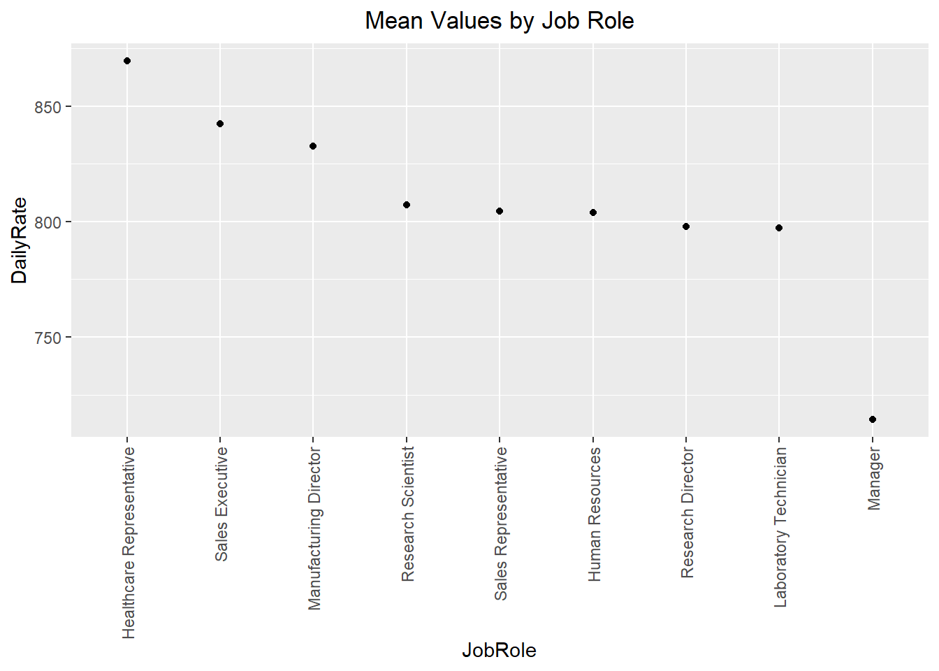
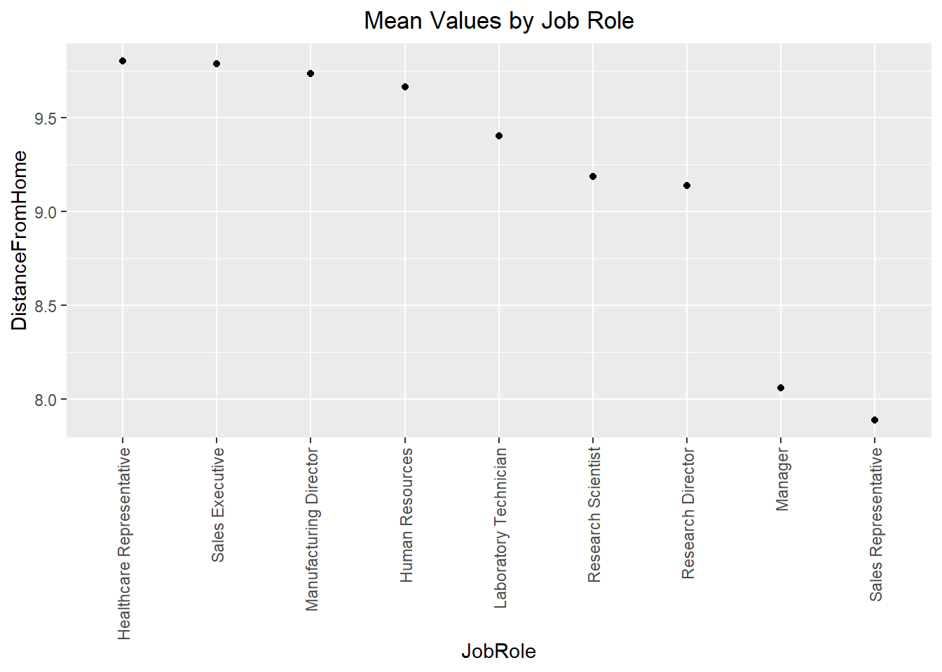
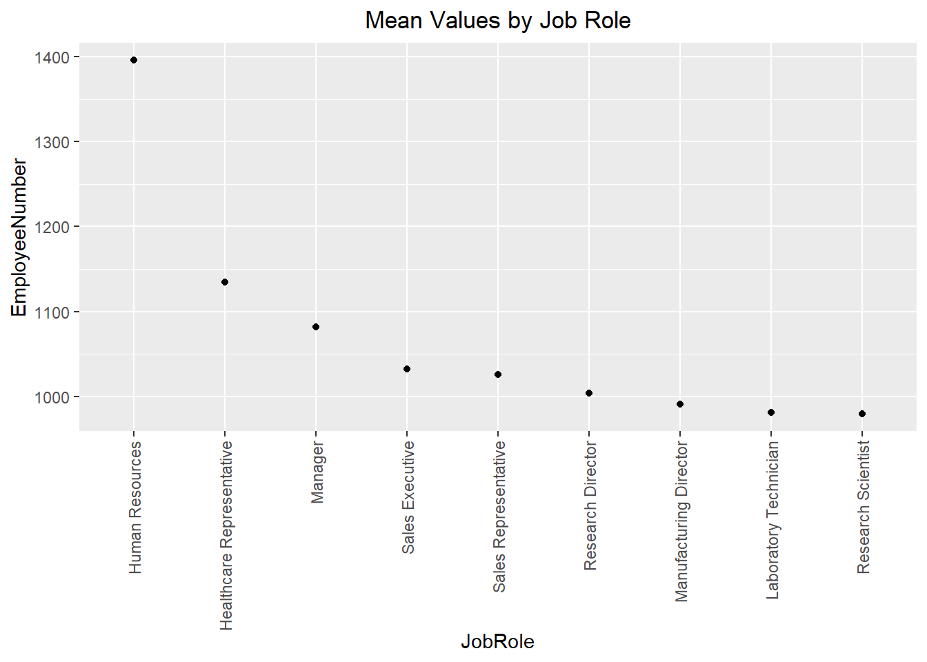
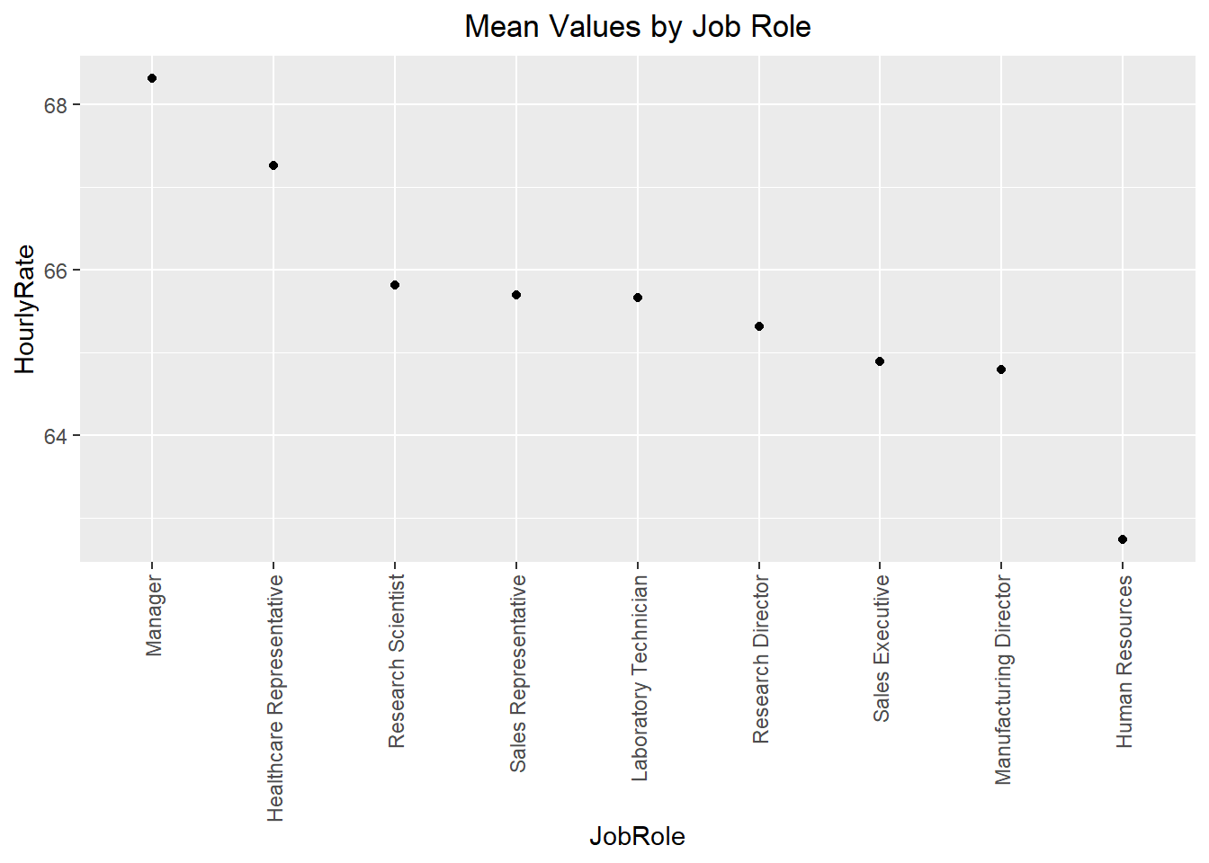
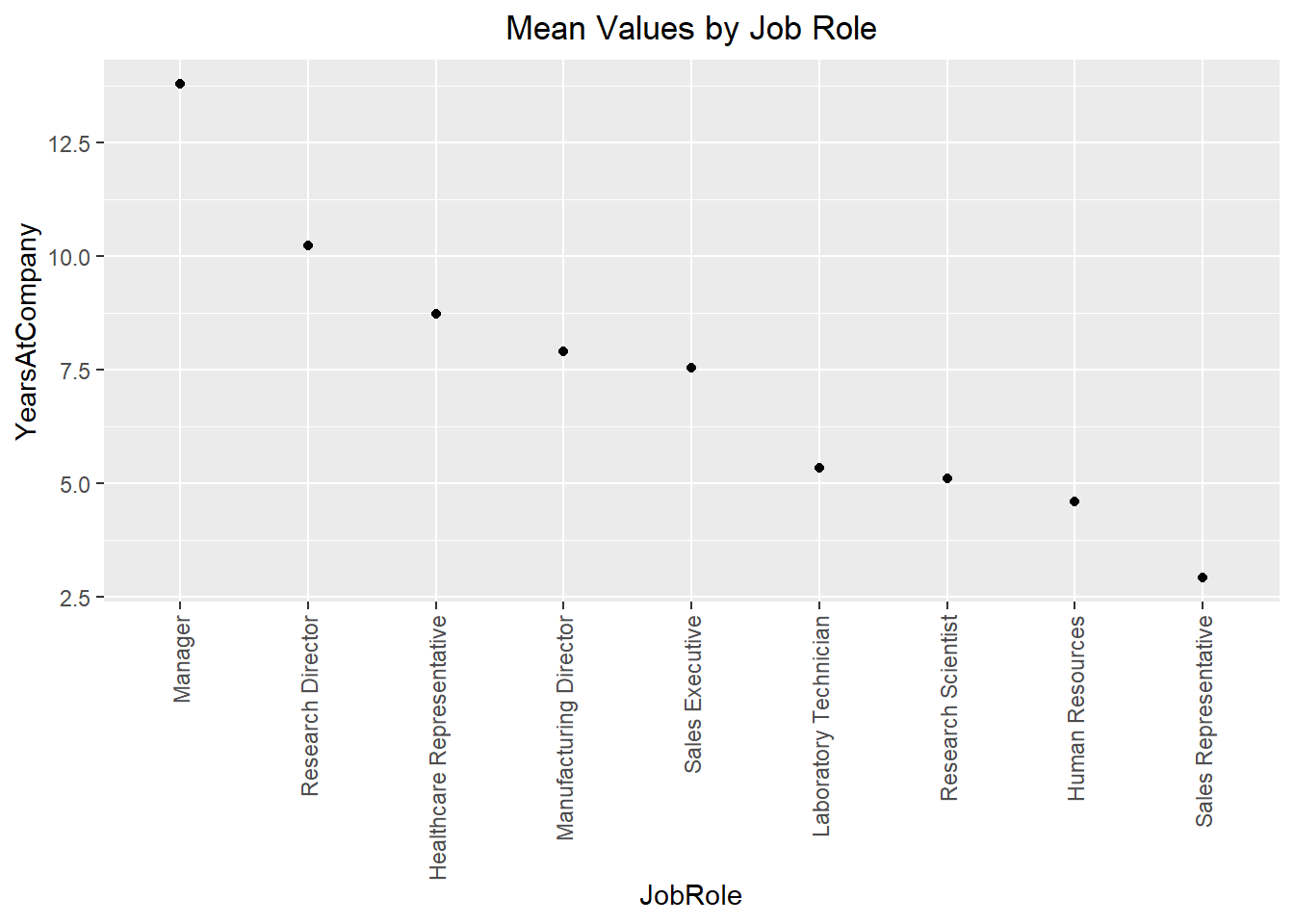
#Factor frequency counts per job role
for (i in 1:length(dfothers)) {

  unq<-data.frame(with(dffactors, table(get(dfothers[i]), JobRole)))

  factorplot <- ggplot(unq, aes(x = reorder(as.factor(get(colnames(unq[2]))), -get(colnames(unq[3]))), y = get(colnames(unq[3])), fill = Var1)) +
    labs(y= colnames(unq[3]), x = colnames(unq[2]), fill= dfothers[i]) +
    geom_bar(position= "stack" , stat="identity") +
    ggtitle('Frequency of Factors by Job Role') + theme(plot.title = element_text(hjust = .5)) +
    theme(axis.text.x = element_text(angle = 90, vjust = 0.5, hjust=1))

  print(factorplot)

}
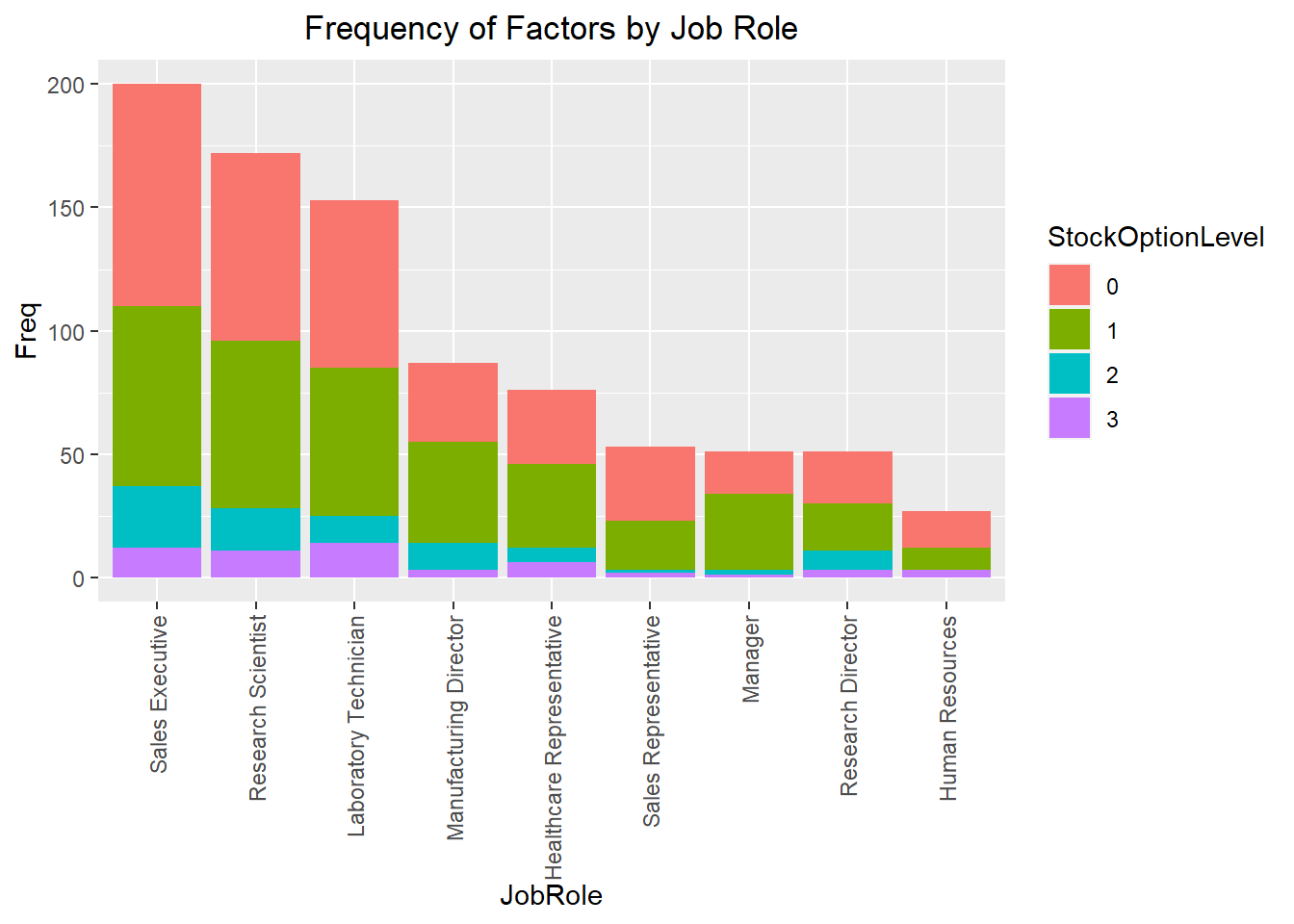
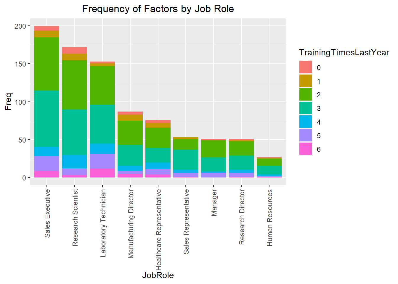
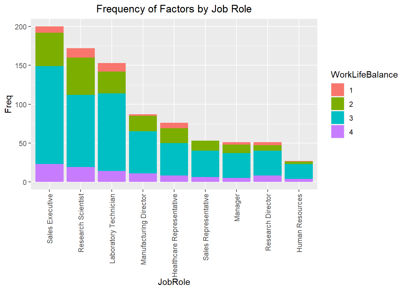
Is the data balanced?
Modeling to predict attrition needs unbiased data. Too many “no” responses. Downsampled to fix.
#check for uneven response variable
kable(table(dffactors$Attrition), col.names = c("Attrition", "Total"))| Attrition | Total |
|---|---|
| No | 730 |
| Yes | 140 |
#downsample to randomly give sample with same number of Yes/No
dflevels <- dffactors[,factorcolumns]
dflevels$Attrition <- dffactors$Attrition
dfNo<- dflevels[which(dflevels$Attrition == "No"),]
dfYes<- dflevels[which(dflevels$Attrition == "Yes"),]
downsamp<-sample(seq(1:length(dfNo$Attrition)), length(dfYes$Attrition))
downsamp <- dfNo[downsamp,]
downsamp <- rbind(downsamp,dfYes)
Find the best randomization seed for splitting our data into training and test sets, and set the seed.
#find best seed for splitting into train and test set
cmloop <- data.frame()
for (i in 1:100) {

  #set seed, take 70% sample and split the data set by the sample data (.7 train/.3 test).
  set.seed(i)
  trainIndicesloop <- sample(seq(1:length(downsamp$Attrition)),round(.7*length(downsamp$Attrition)))
  traindfloop <- downsamp[trainIndicesloop,]
  testdfloop <- downsamp[-trainIndicesloop,]
  testdf2loop <- subset(testdfloop, select = -c(Attrition))

  #NB training model
  trnattrloop = naiveBayes(Attrition~.,data = traindfloop)
  #predict attrition of test set
  nbpredattrloop<-predict(trnattrloop,testdf2loop)
  #make a table of predictions vs actuals
  tblcmloop<-table(nbpredattrloop,testdfloop$Attrition)
  #confusion matrix. columns are actual.
  CM7loop<- caret::confusionMatrix(tblcmloop)
  CM7df1loop<-data.frame(t(CM7loop$overall))
  accloop<-CM7df1loop$Accuracy
  CM7df2loop<-data.frame(t(CM7loop$byClass))
  sensloop<-CM7df2loop$Sensitivity
  specifloop<-CM7df2loop$Specificity
  #build a dataframe from each loop to indicate best seed for training/test split
  cmloop <- rbind(cmloop, data.frame(accloop, sensloop, specifloop))

}

#build a df with the maxmeans
maxmeans <- data.frame(Row = which.max(rowMeans(cmloop)))
maxmeans <- cbind(maxmeans,cmloop[which.max(rowMeans(cmloop)),])

#What row had the highest mean of accuracy + sensitivity + specificity, and what were the values?
kable(maxmeans, col.names = c("Seed", "Accuracy", "Sensitivity", "Specificity"), row.names = F)| Seed | Accuracy | Sensitivity | Specificity |
|---|---|---|---|
| 68 | 0.8333333 | 0.8717949 | 0.8 |
Run the model.
What are conditions with highest probability of predicting Attrition as “yes”?
Accuracy: overall percentage of correct guesses.
Sensitivity: percentage of correct “No” responses.
Specificity: percentage of correct “Yes” responses.
Prediction table helps explain.
#set seed to that row number, which is 68.
set.seed(which.max(rowMeans(cmloop)))

#split the data into training and test set. remove attrition from test set.
trainIndices <- sample(seq(1:length(downsamp$Attrition)),round(.7*length(downsamp$Attrition)))
traindf <- downsamp[trainIndices,]
testdf <- downsamp[-trainIndices,]
testdf2 <- subset(testdf, select = -c(Attrition))

#NB training model and prediction
nbmodel = naiveBayes(Attrition~.,data = traindf, type = "raw")

#Use conditional probabilities to locate highest attrition factors
levelloop <- data.frame()
for (i in 1:length(factorcolumns)) {

  df<-data.frame(nbmodel$tables[i])
  Yes<- df[which(df[1] == "Yes"),]
  Level<- Yes[which(Yes[3] > .2),]
  levelloop <- rbind(levelloop, data.frame(Factor = factorcolumns[i],Level = Level[,2],Probability= Level[,3]))
}

#save our best 3 factors
Topfactors<-tail(levelloop[order(levelloop$Probability),], 3)
kable(Topfactors, row.names = F)| Factor | Level | Probability |
|---|---|---|
| BusinessTravel | Travel_Rarely | 0.6842105 |
| StockOptionLevel | 0 | 0.7157895 |
| PerformanceRating | 3 | 0.8526316 |
#make predictions
preds <- predict(nbmodel, testdf2)

#find out how the model predictions compare to the test dataset actual values.
dfcm <- caret::confusionMatrix(table(preds,testdf$Attrition))
#Accuracy = .833
#Sensitivity = .871
#Specificity = .8
#It did great!
kable(dfcm$table)| No | Yes | |
|---|---|---|
| No | 34 | 9 |
| Yes | 5 | 36 |
#build a df with the maxmeans
dfcmtbl <- data.frame(Accuracy = dfcm$overall[1])
dfcmtbl <- cbind(dfcmtbl, Sensitivity = dfcm$byClass[1])
dfcmtbl <- cbind(dfcmtbl, Specificity = dfcm$byClass[2])

#What were our prediction statistics?
kable(dfcmtbl, row.name = F)| Accuracy | Sensitivity | Specificity |
|---|---|---|
| 0.8333333 | 0.8717949 | 0.8 |
Predicted Classifications
#read in the competition dataset, and wrangle it like our original data but keep the ID column.
compset <- read.csv("CaseStudy2CompSet No Attrition.csv")

compsetresults <- compset

compsetresults[,factorcolumns] <- lapply(compset[,factorcolumns], as.factor)
compsetresults <- compsetresults %>% mutate_if(is.character,as.factor)

#run our model on the dataset, subset it to just IDs and Attrition, and write it to a csv file without rownames.
comppreds <- predict(nbmodel, compsetresults)
compsetresults$Attrition <- comppreds
compsetresults <- subset(compsetresults, select = c(ID, Attrition))
write.csv(compsetresults, file = "Case2PredictionsSherga Attrition.csv", row.names = F)kable(head(compsetresults))| ID | Attrition |
|---|---|
| 1171 | No |
| 1172 | Yes |
| 1173 | No |
| 1174 | No |
| 1175 | No |
| 1176 | No |
Percentage Distribution of Results
histogram(compsetresults$Attrition, xlab = "Attrition Predictions", main = "Classification Results", col = "green")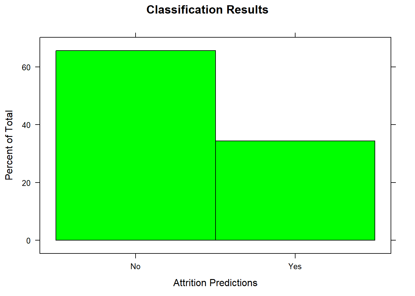
Monthly Income linear model.
Initial model analyses flag insignificant variables on each run, so they can be removed.
Final analysis shows strong significance of these variables as predictors.
#create a new downsampled dataset with a different seed and turn into train and test data.
set.seed(4)
dfNo2<- dffactors[which(dffactors$Attrition == "No"),]
dfYes2<- dffactors[which(dffactors$Attrition == "Yes"),]
downsamp2<-sample(seq(1:length(dfNo2$Attrition)), length(dfYes2$Attrition))
downsamp2 <- dfNo2[downsamp2,]
downsamp2 <- rbind(downsamp2,dfYes2)

trainIndices2 <- sample(seq(1:length(downsamp2$MonthlyIncome)),round(.7*length(downsamp2$MonthlyIncome)))
traindf2 <- downsamp2[trainIndices,]
testdf2 <- downsamp2[-trainIndices,]
testdf3 <- subset(testdf2, select = -c(MonthlyIncome))


salarylm <- lm(MonthlyIncome~., data = traindf2)

#ANOVA to find out which variables are significant in our model.
anva <- anova(salarylm)
#only keep the variables that are 95% significant.
anva <- anva[which(anva$`Pr(>F)` < .05),]
anva
## Analysis of Variance Table
##
## Response: MonthlyIncome
## Df Sum Sq Mean Sq F value Pr(>F)
## Age 1 818358090 818358090 725.2557 < 2.2e-16 ***
## Attrition 1 48400812 48400812 42.8944 1.443e-09 ***
## BusinessTravel 2 11281904 5640952 4.9992 0.0081896 **
## Department 2 90036470 45018235 39.8966 4.663e-14 ***
## Education 4 34249515 8562379 7.5883 1.710e-05 ***
## EducationField 5 47274674 9454935 8.3793 7.734e-07 ***
## EnvironmentSatisfaction 3 23583772 7861257 6.9669 0.0002293 ***
## Gender 1 13643849 13643849 12.0916 0.0007025 ***
## JobInvolvement 3 116299280 38766427 34.3561 3.623e-16 ***
## JobLevel 4 1923827019 480956755 426.2396 < 2.2e-16 ***
## JobRole 8 113855122 14231890 12.6128 4.423e-13 ***
## ---
## Signif. codes: 0 '***' 0.001 '**' 0.01 '*' 0.05 '.' 0.1 ' ' 1#list of significant variables, and include MonthlyIncome.
sigterms <- tidy(anva)$term
sigterms[nrow(as.data.frame(sigterms)) + 1] <- "MonthlyIncome"
salarylm <- lm(MonthlyIncome~., data = traindf2[,sigterms])
anva <- anova(salarylm)
anva <- anva[which(anva$`Pr(>F)` < .05),]
anva## Analysis of Variance Table
##
## Response: MonthlyIncome
## Df Sum Sq Mean Sq F value Pr(>F)
## Age 1 818358090 818358090 709.9177 < 2.2e-16 ***
## Attrition 1 48400812 48400812 41.9872 1.068e-09 ***
## BusinessTravel 2 11281904 5640952 4.8935 0.0086473 **
## Department 2 89914963 44957482 39.0002 1.543e-14 ***
## Education 4 34643268 8660817 7.5132 1.420e-05 ***
## EducationField 5 46104180 9220836 7.9990 9.293e-07 ***
## EnvironmentSatisfaction 3 27205804 9068601 7.8669 6.245e-05 ***
## Gender 1 13831933 13831933 11.9991 0.0006821 ***
## JobInvolvement 3 118307357 39435786 34.2102 < 2.2e-16 ***
## JobLevel 4 1924154661 481038665 417.2963 < 2.2e-16 ***
## JobRole 8 104230699 13028837 11.3024 1.216e-12 ***
## ---
## Signif. codes: 0 '***' 0.001 '**' 0.01 '*' 0.05 '.' 0.1 ' ' 1#all remaining variables are significant
#display all best predictors
predtbl<-data.frame(Predictors = tidy(anva)$term)
predtbl$`P-Values` <- anva$`Pr(>F)`
kable(predtbl)| Predictors | P-Values |
|---|---|
| Age | 0.0000000 |
| Attrition | 0.0000000 |
| BusinessTravel | 0.0086473 |
| Department | 0.0000000 |
| Education | 0.0000142 |
| EducationField | 0.0000009 |
| EnvironmentSatisfaction | 0.0000625 |
| Gender | 0.0006821 |
| JobInvolvement | 0.0000000 |
| JobLevel | 0.0000000 |
| JobRole | 0.0000000 |
Use linear model to make prediction on test set.
RMSE tells deviation from our model in dollars.
Here we can see the RMSE when the model is run on our test, training, and full datasets.
#use model to make prediction on our test set.
lmpreds <- predict(salarylm, testdf3)
#calculate the error by finding the difference between predictions and actuals. then calculate the root mean square error.
err <- lmpreds - testdf2$MonthlyIncome
RMSEdf <- data.frame(Test_RMSE = sqrt(mean(err^2)))
#RMSE = $1200.833 monthly income

lmpredstrain <- predict(salarylm, traindf2)
#calculate the error by finding the difference between predictions and actuals. then calculate the root mean square error.
errtrain <- lmpredstrain - traindf2$MonthlyIncome
RMSEdf$Train_RMSE <- sqrt(mean(errtrain^2))
#RMSE = $973.089 monthly income

lmpredfull <- predict(salarylm, dffactors)
#calculate the error by finding the difference between predictions and actuals. then calculate the root mean square error.
errfull <- lmpredfull - dffactors$MonthlyIncome
RMSEdf$Full_RMSE <- sqrt(mean(errfull^2))
#RMSE = $1064.57 monthly income

kable(RMSEdf, col.names = c("Test RMSE", "Train RMSE", "Full RMSE"))| Test RMSE | Train RMSE | Full RMSE |
|---|---|---|
| 1200.833 | 973.0891 | 1064.569 |
Residual Plot
Plot predicted values vs actual to observe residuals on zero line.
Random scattering on both sides of the reference line.
#plot model predictions compared to actuals, in order to see regression trend.
plot(lmpreds,testdf2$MonthlyIncome,
     xlab = "Predicted Monthly Income",ylab = "Actual Monthly Income", main = "Linear Comparison of Predictions vs Actuals")
abline(a = 0, b = 1)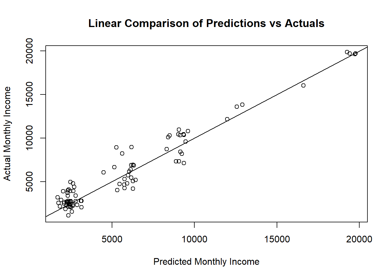
#plot model predictions compared to actuals, in order to see regression trend.
plot(lmpredstrain,traindf2$MonthlyIncome,
     xlab = "Predicted Monthly Income",ylab = "Actual Monthly Income", main = "Linear Comparison of Predictions vs Actuals")
abline(a = 0, b = 1)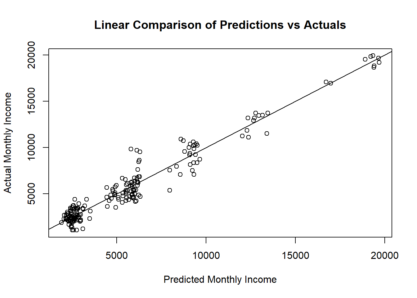
#plot model predictions compared to actuals, in order to see regression trend.
plot(lmpredfull,dffactors$MonthlyIncome,
     xlab = "Predicted Monthly Income",ylab = "Actual Monthly Income", main = "Linear Comparison of Predictions vs Actuals")
abline(a = 0, b = 1)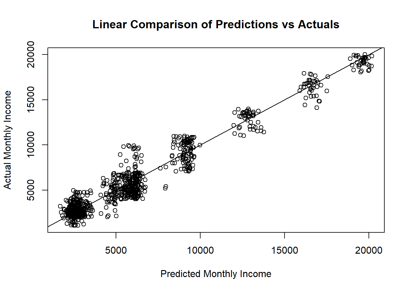
Predicted Monthly Incomes
#read in the competition dataset, and wrangle it like our original data but keep the ID column.
salcompset <- read_xlsx("CaseStudy2CompSet No Salary.xlsx")

salcompsetresults <- salcompset

salcompsetresults[,factorcolumns] <- lapply(salcompset[,factorcolumns], as.factor)
salcompsetresults <- salcompsetresults %>% mutate_if(is.character,as.factor)


#run our model on the dataset, subset it to just IDs and monthlyincome, and write it to a csv file without rownames.
salcomppreds <- round(predict(salarylm, salcompsetresults), digits = 2)
salcompsetresults$MonthlyIncome <- salcomppreds
salcompsetresults <- subset(salcompsetresults, select = c(ID, MonthlyIncome))
write.csv(salcompsetresults, file = "Case2PredictionsSherga Salary.csv", row.names = F)kable(head(salcompsetresults))| ID | MonthlyIncome |
|---|---|
| 871 | 6006.17 |
| 872 | 2701.10 |
| 873 | 13049.47 |
| 874 | 2757.69 |
| 875 | 2626.98 |
| 876 | 4174.28 |
Percentage Distribution of Results
Similar shape to downsampled dataset.
hist(salcompsetresults$MonthlyIncome, xlab = "Monthly Income Predictions", main = "Prediction Results",  col = "green", prob = TRUE)
lines(density(salcompsetresults$MonthlyIncome, adjust = 2))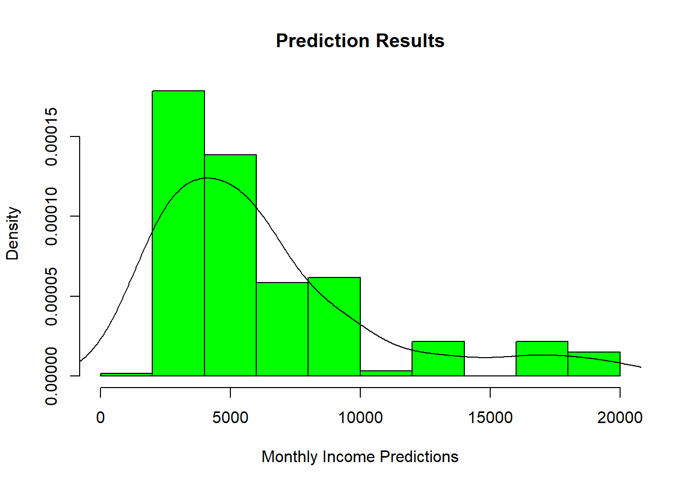
hist(downsamp2$MonthlyIncome, xlab = "Source data", main = "Downsampled Data Income",  col = "green", prob = TRUE)
lines(density(downsamp2$MonthlyIncome))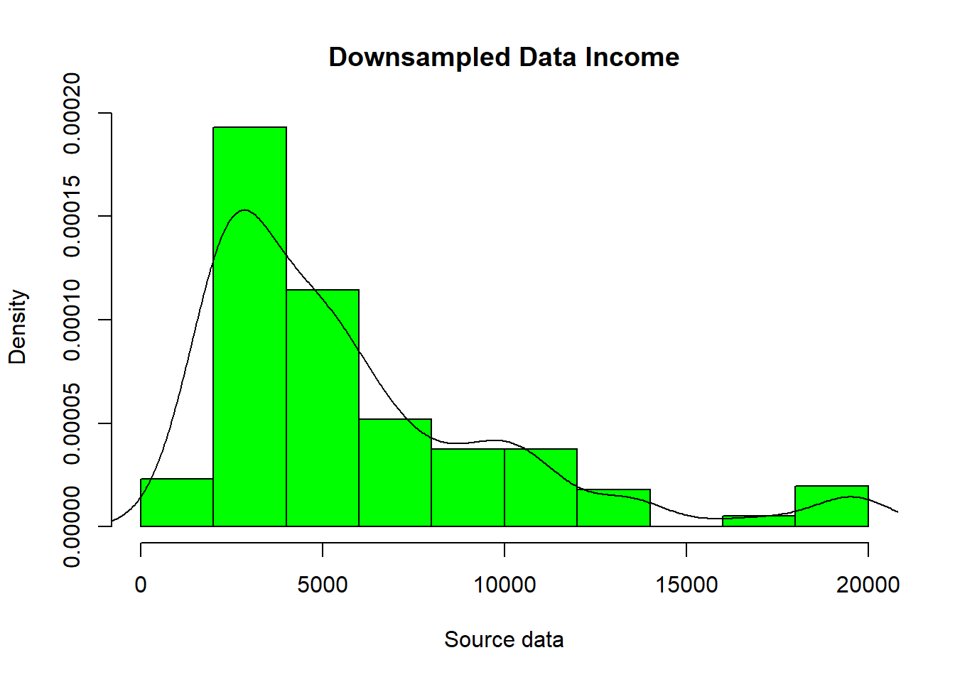
PowerPoint Slides